1. Version Management
Updated Description Sheet
Version Description Date
| V2.6.4 | 1. Removed: Fan Control section | 07/16/2026 | |
|---|---|---|---|
| 2. Added: Phase Modulation section | |||
| 3. Added: Compact Mode (Minibar) section | |||
| 4. Added: Frequency and Power Settings section | |||
| 5. Added: Medium-Power Output (Option 10) section | |||
| 6. Removed: Default update method in the Software and | |||
| Firmware Update section |
V2.6.4 1. Removed: Fan Control section
07/16/2026
2. Added: Phase Modulation section
3. Added: Compact Mode (Minibar) section
4. Added: Frequency and Power Settings section
5. Added: Medium-Power Output (Option 10) section
6. Removed: Default update method in the Software and
Firmware Update section
V2.6.2 1. Removed: Streaming Mode section
06/16/2026
2. Refactored: Introduction to Operating Modes section
3. Added: Quick Waveform section
4. Added: Multitone section
| V2.5.4 | 1. Added: Connect ETH Device section | 05/09/2026 | ||||
|---|---|---|---|---|---|---|
| 2. Added: External Reference Clock Input section | ||||||
| 3. Added: Reference Clock Output section | ||||||
| 4. Added: Trigger Input section | ||||||
| 5. Added: Trigger Output section | ||||||
| 6. Added: RF Hardware section | ||||||
| 7. Added: GNSS Usage section | ||||||
| 8. Refactored: RF and Modulation Control section | ||||||
| 9. Added: Software and Firmware Update section | ||||||
| V1.1.5 | 1. Initial Version | 03/19/2026 |
V2.5.4 1. Added: Connect ETH Device section
05/09/2026
2. Added: External Reference Clock Input section
3. Added: Reference Clock Output section
4. Added: Trigger Input section
5. Added: Trigger Output section
6. Added: RF Hardware section
7. Added: GNSS Usage section
8. Refactored: RF and Modulation Control section
9. Added: Software and Firmware Update section
V1.1.5 1. Initial Version 03/19/2026
1
2. System Requirements
The VSG-mini-6 is a USB vector signal generator, and the accompanying software needs to be
installed and run on a host PC. The recommended host PC operating environment is shown in
the table below.
The table only lists the basic recommended configurations. For systems below the
recommended specifications, please refer to the actual test results.
Table 1 System Operating Environment Requirements
| Operating System | Windows 11/10/8/7, dependent on VS2019 C++ redistributables |
|---|---|
| Architecture | Windows: x64 |
Operating System Windows 11/10/8/7, dependent on VS2019 C++ redistributables
Architecture Windows: x64
Processor Intel i3 or above
8 GB RAM.
Memory
If generating digitally modulated waveforms with PN > 15, 16 GB RAM is
recommended to improve performance and processing capability
Storage If outputting 62.5 MHz sample rate signals in streaming mode, the hard
drive must support a sustained read/write speed greater than 250 MB/s
| Data Interface | USB 2.0 or USB 3.0 (USB 3.0 recommended) Streaming mode is limited by the bandwidth of the data interface | |
|---|---|---|
| Display Resolution | At least 1280 × 800 pixels | |
| Other | Some antivirus software may prevent the system from operating normally |
Data Interface USB 2.0 or USB 3.0 (USB 3.0 recommended)
Streaming mode is limited by the bandwidth of the data interface
Display Resolution At least 1280 × 800 pixels
Other Some antivirus software may prevent the system from operating
normally
2
3. Introduction to Operating Modes
The system supports multiple signal generation modes, including CW, AM, FM, PM, pulse,
digital ramp sweep, Gaussian white noise, digital modulation, DSSS, OFDM, playback, multitone,
streaming mode, and quick waveform generation. This chapter describes in detail the
configuration methods and underlying signal generation mechanisms of these operating
modes.
3.1 Overview of Operating Modes
In actual hardware operation, the above modes are primarily based on three underlying
operating methods: CW, onboard memory playback, and high-speed real-time streaming.
Please select the appropriate operating mode according to your test requirements.
Table 2 Operating Environment Requirements
Operating Method Corresponding
Software Button/Mode Description
| CW Mode | RF On Only | The hardware directly and continuously | |
|---|---|---|---|
| transmits a CW signal without occupying | |||
| waveform memory. |
The hardware directly and continuously transmits a CW signal without occupying waveform memory.
CW Mode RF On Only
The core operating mode of the system. The
AM, FM, PM, Pulse,
software either generates IQ data blocks
Digital Ramp Sweep,
based on parameters or imports user-
AWGN, DSSS, OFDM,
Playback Mode
provided IQ data (up to 125 MB), downloads
Digital Modulation,
them to the device’s onboard memory in a
Playback, Quick Wave,
single transfer, and the hardware timer then
Multitone
drives looped or single-shot transmission.
Bypasses the onboard storage capacity
limitation. Real-time generated IQ data
streams are continuously and dynamically
Streaming Mode Streaming Mode
transferred to the transmission engine
through a high-speed bus, making it suitable
for ultra-long-duration signal simulation.
3.2 CW Mode
When RF output is enabled and modulation is disabled in the software interface, the device
enters CW mode. In this mode, a single-tone carrier signal can be generated without loading
any baseband waveform file.
3
3.3 Playback Mode
This mode adopts an onboard memory preloaded playback mechanism. When the signal type
or parameters are modified, the host software immediately calculates and generates the
corresponding IQ data and downloads the complete waveform into the instrument’s internal
memory. Since the waveform data is preloaded and resides entirely within the hardware,
transmission does not rely on real-time bus transfer, enabling stable output at the instrument’s
maximum supported analog bandwidth (100 MHz).
Amplitude Modulation
In AM mode, the instrument modulates the amplitude of a high-frequency carrier using a low-
frequency baseband signal. This mode is commonly used for wireless communications,
broadcast receiver testing, and modulation characteristic analysis. The AM mode provides the
following functions:
- AM parameter configuration
- Baseband IQ data export
Frequency Modulation
In FM mode, the instrument modulates the instantaneous frequency of a high-frequency carrier
using a low-frequency modulation waveform. Modulation types such as sine wave, square
wave, triangle wave, and ramp wave are supported. This mode is widely used for testing walkie-
talkies, vehicle-mounted radios, and wireless communication equipment. The FM mode
provides the following functions:
- FM parameter configuration
- Baseband IQ data export
Phase Modulation
In Phase Modulation (PM) mode, the instrument modulates the instantaneous phase of the RF
carrier according to the selected modulation waveform. It supports sine, square, triangle, and
ramp modulation waveforms, with configurable modulation rate, phase deviation, and initial
phase. This mode is suitable for testing communication systems, receivers, and phase
modulation characteristics. The Phase Modulation mode provides the following functions:
- PM parameter configuration
- Baseband IQ data export
Pulse
In Pulse mode, the instrument generates pulse-modulated signals by applying gating control
to the RF carrier. This mode is suitable for receiver transient response testing, pulsed
characteristic testing of microwave devices, as well as radar and navigation system excitation
applications. The Pulse mode provides the following functions:
4
- Pulse parameter configuration
- Baseband IQ data export
Digital Ramp Sweep
In Digital Ramp Sweep mode, the output frequency performs linear frequency sweeping
according to the configured sweep span, sweep time, and sweep period. The instrument
achieves high-precision frequency ramp generation through digital frequency control, making
it suitable for applications such as radar linear frequency modulation (LFM) signal simulation,
broadband excitation, and frequency response testing. This mode provides the following
functions:
- Sweep parameter configuration
- Baseband IQ data export
AWGN
In AWGN mode, the instrument outputs broadband noise signals within a specified bandwidth
range, with amplitude statistical characteristics following a Gaussian distribution. This mode is
commonly used for receiver anti-interference testing, SNR testing, and system noise
performance evaluation. The mode provides the following functions:
- Bandwidth and length configuration
- Baseband IQ data export
Digital Modulation
In Digital Modulation mode, the instrument maps baseband digital bit streams onto IQ
constellation points and outputs the signals after pulse-shaping filtering. The Digital
Modulation mode provides the following functions:
- Digital Mod Parameter configuration
- ASK/APSK/FSK/PSK/QAM modulation
- Raw baseband IQ data export
- Data truncation and parameter
adjustment
- IQ/spectrum/constellation diagram
preview
DSSS
In DSSS mode, the instrument performs spread-spectrum processing on baseband modulated
data using pseudo-random spreading codes, thereby expanding the signal spectrum. This
mode supports spreading code configuration, random seed settings, and pulse-shaping filter
configuration, making it suitable for spread-spectrum communication systems and anti-
interference testing. The DSSS mode provides the following functions:
- DSSS core parameter configuration
- Raw baseband IQ data export
5
OFDM
In OFDM mode, the instrument maps data streams onto multiple mutually orthogonal
subcarriers for parallel modulation, thereby generating broadband multicarrier communication
signals. This mode supports configuration of parameters such as FFT length, guard interval,
subcarrier allocation, and modulation type, making it suitable for wireless communication
systems, receiver performance evaluation, and spectrum characteristic testing. The OFDM
mode provides the following functions:
- Basic OFDM parameter configuration
- OFDM time-frequency structure
configuration
- Raw baseband IQ data export
Multitone
In Multitone mode, the instrument supports the generation of multiple discrete tones with equal
frequency spacing to meet the requirements of receiver testing, intermodulation testing,
linearity testing, and complex spectrum scenario simulation. The Multitone mode provides the
following functions:
- Multitone signal generation
- Individual tone enable/disable control
- Fixed, random, and parabolic phase
- In-band notch function
control
Playback
In Playback mode, the instrument supports downloading user-provided external waveform
data in .wav format (up to 125 MB) into the instrument’s internal memory for transmission,
meeting the requirements of complex non-standard protocols or custom signal generation
applications. The Playback mode provides the following functions:
- Single external waveform file loading
- Real-time waveform parameter parsing
- Playback sample count and range
- IQ amplitude control and automatic scaling
control
Quick Waveform
In Quick Waveform mode, the instrument allows users to directly replay built-in modulation
waveform files, eliminating the need for complex parameter configuration and external file
import procedures, and enabling one-click generation of standard signals. The Quick
Waveform mode provides the following functions:
6
- Preset waveform files
- Real-time waveform parameter parsing
- IQ amplitude control and automatic scaling
- Playback sample count and range
control
3.4 Streaming Mode
In this mode, the software transmits IQ waveform data to the instrument via the USB bus. The
instrument receives the data and plays it in real time. When the user stops streaming data, the
instrument continues playback until all received data has been played, and then stops. The
sampling rate and transmission rate of real-time data are limited by the physical bandwidth of
the data interface. The streaming mode in the software uses this transmission mechanism.
- Loading multiple waveform files
- File parameter parsing
- Playback progress display
- IQ amplitude control
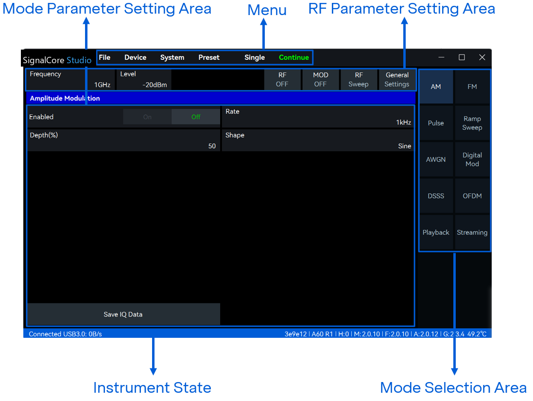
3.5 Interface Layout
The SignalCore Studio interface consists of the following components:
- Menu
- RF Parameter Settings Area
- Mode Selection Area
- Mode Parameter Settings Area
- Instrument State
Figure 1 SignalCore Studio Interface Layout
7
Menu
- Save and Open Configuration Files
- Set Power On State
- Connect USB/ETH devices
- Switch language/theme
- Preference settings
- GNSS Information
- View instrument information
- Software and firmware update
- Preset
- Single and continuous transmission
RF Parameter Settings Area
- Frequency
- Level
- RF On/Off
- Modulation On/Off
- Frequency/Power Sweep
- General Settings
Mode Selection Area
- AM
- FM
- PM
- Pulse
- Digital Ramp
- AWGN
- Digital Mod
- DSSS
- OFDM
- Playback
- Streaming
- Multitone
- Quick Waveform
Instrument State
- Instrument Connection Status
- Bus Data Throughput
- Instrument Model and UID
- Software/Firmware Version
- Instrument Real-Time Temperature
8
4. General Operations
4.1 Save and Open Configuration Files
1. Save Current Configuration
1). Click "File" -> "Save" in the menu bar;
2). In the "Save Settings" dialog, set the save path and file name, then click "Save". Instrument
configuration files are saved in the "/data" folder by default.
2. Load Preset Configuration
1). Click "File" -> "Open" in the menu bar;
2). In the "Open Settings" dialog, select the configuration file and click "Open" to apply the
preset configuration.
4.2 Set Power On State
The instrument supports user-defined startup states. Detailed description of the available
power on state is provided in the table below.
Table 3 SignalCore Studio Software Power On State
No. Power On State Name Description
1 Default Instrument default configuration
2 User Preset Use a user-saved configuration file as the initial power on
configuration
3 Last State Use the parameter configuration from the previous
software session as the initial startup configuration
To set the startup state, follow these steps:
1. Click "File" -> "Power On State" in the menu bar;
2. For "Default" or "Last State", just click the option. The software will use the selected option
as the initial state on the next startup;
3. Select "User Preset" and choose a user-saved configuration file in the "Open Settings"
dialog. The software will open with this specified configuration on the next startup.
1
4.3 Connect USB Device
When the instrument is directly connected to the computer via a USB cable, click "Device" ->
"USB Connect" in the menu bar. The interface will display a list of all signal generators connected
to the PC, click the first six digits of the corresponding UID to switch the currently connected
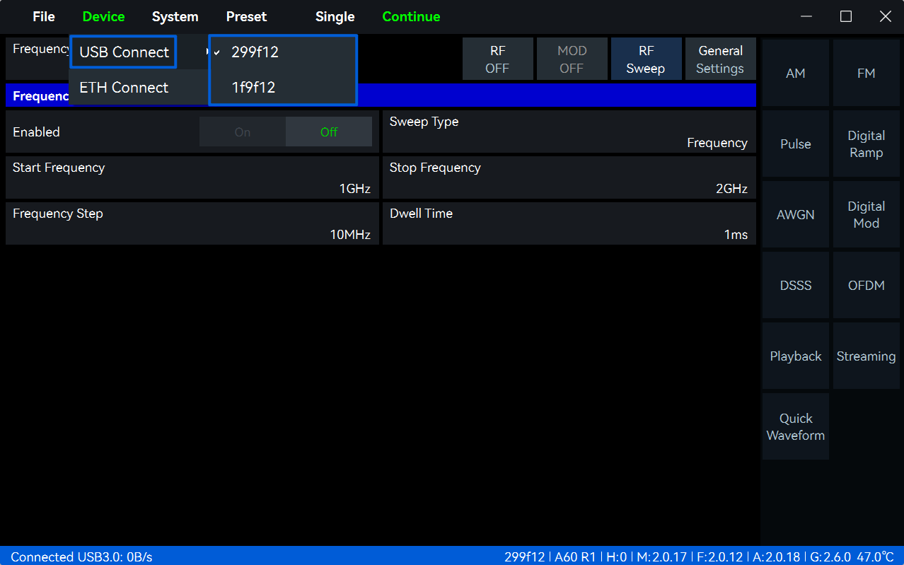
instrument.
Figure 2 Connect the USB device
4.4 Connect ETH Device
1. When using an Ethernet-based instrument, navigate to the menu bar and select "Device" ->
"ETH Connect". In the dialog box, enter the "IP Address" and "Port", then select the "Local
Interface" (ensure the PC is configured to the same network segment as the instrument);
2. Click "Connect". The software will attempt to establish a connection with the device. Once
successful, the status bar will display "Connected ETH XXX" (e.g., Connected ETH
192.168.1.100 0 B/s).
4.5 Theme Setting
Click "System" -> "Theme" in the menu bar to switch between the "Dark" and "Light" themes.
4.6 Preference Settings
Click "System" -> "Preference" in the menu bar to open the configuration window. The following
functional settings can be configured.
2
Table 4 Preference Settings Description
Parameter Description
Screen Lock On: A lock icon" " will appear on the right side of the screen. Click
the icon" " to lock the screen and prevent accidental operations;
click again to unlock.
Auto Mod On: When "Enable" in the mode parameter settings area is selected,
the "Modulation" control in the RF parameter settings area will be
automatically enabled, with no manual operation required.
Off: The "MOD" control in the RF parameter settings area must be
enabled manually.
4.7 Viewing Instrument Information
Click "System" -> "About" in the menu bar. A dialog box will display information such as the
current instrument's UID, software/firmware version, power port voltage and current, and USB
port voltage and current.
4.8 Single and Continuous Transmission
Single: Click "Single" to transmit the signal once;
Continue: Click "Continue" to transmit the signal continuously.
4.9 Preset
Click the "Preset" button in the menu bar to restore the current software configuration to the
instrument's default initial state.
4.10 Compact Mode (Minibar)
Compact Mode switches the software main interface to a simplified quick control panel while
retaining commonly used functions such as RF output, output frequency, output power,
modulation, and frequency/power sweep. It enables users to quickly configure key parameters
when working with multiple application windows.
1. Click the " " icon on the menu bar to switch the software to the Compact Control Panel;
2. Set the output frequency and output power, then enable RF Output to quickly generate a
CW signal;
3. To output a modulated signal or perform a frequency/power sweep, click the "Mod" or
"Frequency/Power Sweep" button to expand the corresponding parameter configuration
panel. After completing the configuration, click anywhere outside the panel to collapse it;
4. Click "Restore" to exit Compact Mode and return to the main software interface. Click the "
/ " toggle button at the bottom of the panel to collapse or expand the Compact Control
Panel.
3
Note: The parameter settings, valid ranges, and application methods in Compact Mode are
identical to those in the main software interface. For detailed descriptions, refer to the
corresponding functional sections.
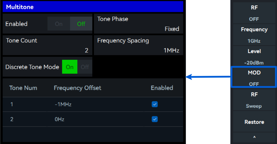
figure 3 Launch Minibar and configure the parameters
4.11 Frequency and Power Settings
The output frequency and peak power can be configured at the top of the software main
interface. Based on the current configuration, the instrument returns the corresponding RMS
power value. The parameters are described in the table below.
Table 5 Frequency and Power Settings
Frequency and Power
| Frequency | Sets the output frequency of the RF signal. Range: 9 kHz to 6 GHz. | |
|---|---|---|
| For output frequencies below 500 MHz, the frequency resolution | ||
| is 1 Hz. | ||
| For output frequencies from 500 MHz to 6 GHz, the frequency | ||
| resolution is 0.1 Hz. |
Sets the output frequency of the RF signal. Range: 9 kHz to 6 GHz.
For output frequencies below 500 MHz, the frequency resolution
Frequency
is 1 Hz.
For output frequencies from 500 MHz to 6 GHz, the frequency
resolution is 0.1 Hz.
Sets the peak output power of the signal. The standard
Power
configuration provides a maximum output power of 7 dBm to 14
dBm, with an optional 25 dBm high-power output.
| RMS | Displays the actual average power of the current output signal. | |
|---|---|---|
| This is a read-only value and cannot be configured. |
RMS Displays the actual average power of the current output signal.
This is a read-only value and cannot be configured.
4.12 Medium-Power Output (Option 10)
The instrument supports an optional Medium-Power Output (Option 10). When this option is
installed, the maximum output power is increased to 25 dBm, and signals are output through
the dedicated medium-power RF output port. To output a medium-power RF signal:
4
1. Click "General Settings" in the RF Control section, and set "Output Port" to "HP Port" under
the RF Hardware settings;
2. Connect the RF cable to the instrument's medium-power RF output port;
3. Configure the desired output frequency, output power, and signal type, then enable "RF-
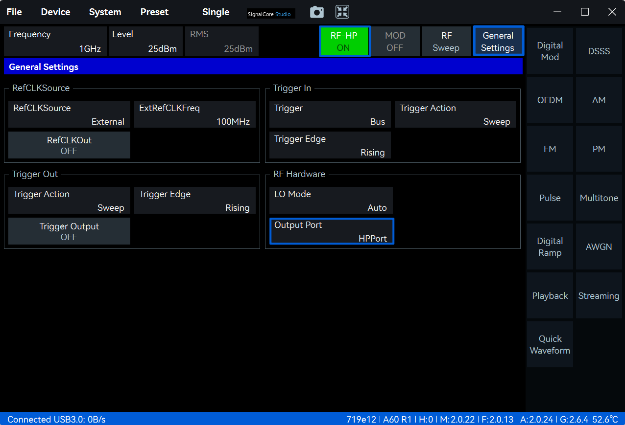
HP" to output the configured signal.
figure 4 25 dBm CW Signal Output via the Medium-Power Port
4.13 RF and Modulation Control
During a Frequency Sweep or Power Sweep, modulation can be enabled concurrently, allowing
the modulated signal to track variations in frequency or power. The functions of the RF and
Modulation control button are detailed in the table below:
Table 6 RF and Modulation
RF and Mod Control
RF ON/OFF Controls the RF output state. When set to "OFF", the RF output is
forcibly disabled regardless of other settings.
| MOD ON/OFF | Switches the current modulation state. | |
|---|---|---|
| When MOD is set to "OFF" and RF is set to "ON", the instrument | ||
| outputs a CW signal. | ||
| When both states are "ON", the instrument outputs the signal using | ||
| the currently selected modulation type. |
Switches the current modulation state.
When MOD is set to "OFF" and RF is set to "ON", the instrument
MOD ON/OFF
outputs a CW signal.
When both states are "ON", the instrument outputs the signal using
the currently selected modulation type.
5
4.14 Frequency and Power Sweep
When only RF and Frequency/Power Sweep are enabled, the instrument outputs a CW sweep
signal. By additionally enabling the MOD function, the instrument provides a modulated sweep
signal output.
Parameter Description
Table 7 Frequency and Power Sweep Parameter Description
Frequency and Power
Sweep (Analog)
| Sweep Type | Frequency Sweep: Sweeps the frequency across the specified | |
|---|---|---|
| range at a fixed level; | ||
| Power Sweep: Sweeps the level across the specified range at a | ||
| fixed frequency. | ||
| Start/Stop Frequency | Sets the sweep range for frequency sweep. | |
| Start/Stop Level | Sets the sweep range for power sweep. | |
| Frequency Step | Sets the frequency step size between adjacent sweep points in | |
| frequency sweep. | ||
| Level Step | Sets the level increment between adjacent sweep points in level | |
| sweep. | ||
| Dwell Time | Sets the update interval between adjacent sweep points. The | |
| actual interval is the sum of the instrument reconfiguration time | ||
| and the dwell time at each frequency/level point. Range: 1 ms to | ||
| 1000 s. |
Frequency Sweep: Sweeps the frequency across the specified
range at a fixed level;
Sweep Type
Power Sweep: Sweeps the level across the specified range at a
fixed frequency.
Start/Stop Frequency Sets the sweep range for frequency sweep.
Start/Stop Level Sets the sweep range for power sweep.
Frequency Step Sets the frequency step size between adjacent sweep points in
frequency sweep.
Level Step Sets the level increment between adjacent sweep points in level
sweep.
Sets the update interval between adjacent sweep points. The
actual interval is the sum of the instrument reconfiguration time
Dwell Time
and the dwell time at each frequency/level point. Range: 1 ms to
1000 s.
Operating Procedure
Using an analog frequency sweep signal with a start frequency of 1 GHz, stop frequency of 2
GHz, power level of -20 dBm, frequency step of 100 MHz, and dwell time of 10 ms as an example,
the operation procedure is as follows:
1. Click "RF Sweep" in the RF parameter settings area;
2. In the parameter settings area, set "Sweep Type" as "Frequency", "Start Frequency" as 1
GHz, "Stop Frequency" as 2 GHz, "Frequency Step" as 100 MHz, and "Dwell Time" as 10 ms,
then enable the RF Sweep mode;
3. Set the Level to -20 dBm, and set the RF On;
4. The signal generator outputs an analog frequency sweep signal with a start frequency of 1
GHz, stop frequency of 2 GHz, level of -20 dBm, frequency step of 100 MHz, and dwell time
of 10 ms.
6
4.15 External Reference Clock Input
1. Refer to the Vector Signal Generator Quick Start Guide to input an external reference
clock.
2. Click "General Settings" -> "RefCLKSource", and select "External". Set the Reference Clock
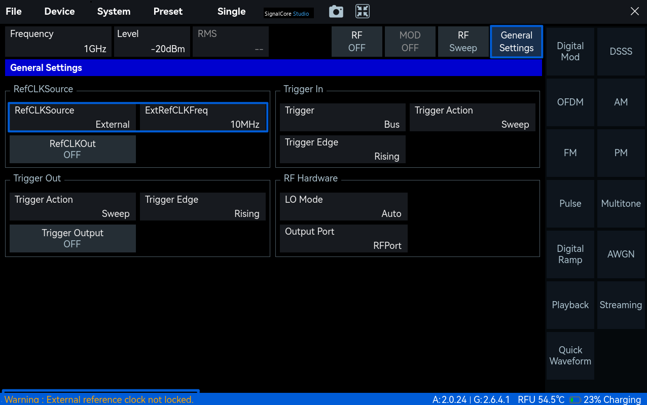
Frequency as 10 MHz. If the status bar at the bottom displays the warning message
"Warning: External reference clock not locked", the switch to the external reference clock
has failed. If no such warning is displayed, the switch has been completed successfully.
figure 5 Reference Clock Switching Failure
4.16 Reference Clock Output
1. Refer to the Vector Signal Generator Quick Start Guide and connect the instrument's
reference clock output port.
2. Click "General Settings" in the RF parameter settings area and enable "RefCLKOut" to
output a 100 MHz clock signal.
7
4.17 Trigger Input
Parameter Description
Table 8 Trigger Input Parameter Description
Trigger Input
Trigger Source Supports bus trigger, external trigger, and XPPS trigger.
The trigger action takes effect only when RF sweep is enabled.
Sweep: Upon receiving a trigger signal, the instrument starts the
preset RF sweep. During the sweep process, the switching interval
between adjacent RF sweep points is determined by the dwell time.
Trigger Action
Hop: Upon receiving a trigger signal, the system performs only a
single-step transition and switches to the next RF state in the
preset sweep sequence. In this mode, the dwell time is ignored, and
the hopping rate depends on the arrival rate of the trigger pulses.
Trigger Edge Supports both rising edge and falling edge triggering. In Bus trigger
mode, the trigger edge setting is ignored.
Operating Procedure
Using an AM signal with frequency hopping as an example, the operation procedure is as
follows:
1. Refer to the Vector Signal Generator Quick Start Guide to configure the external trigger
input;
2. Click "AM" in the mode selection area. In the mode parameter configuration area, set
"Rate" to 200 kHz, keep the remaining parameters at their default values, and enable AM
mode;
3. In the RF parameter settings area, click "RF Sweep". In the mode parameter configuration
area, set "Frequency Step" to 100 MHz, keep the remaining parameters at their default
values, and enable the RF Sweep mode;
4. Click "General Settings" in the RF parameter configuration area, set "Trigger Source" to
"External", and set "Trigger Action" to "Hop";
5. Enable the RF output. The instrument then enters the trigger-wait state. Each time a valid
external trigger is received, the system hops to the next frequency point with a 100 MHz
step size and simultaneously outputs an AM signal with a modulation rate of 200 kHz.
8
4.18 Trigger Output
Table 9 Trigger Output Parameter Description
Trigger Output
Trigger Output Enable or disable the trigger output function.
| Trigger Action | Sweep: Outputs one trigger signal after completing one RF sweep; Hop: Outputs one trigger signal after completing one frequency hop. | |
|---|---|---|
| Trigger Edge | The output trigger can be configured as either a rising edge or falling | |
| edge. |
Trigger Action Sweep: Outputs one trigger signal after completing one RF sweep;
Hop: Outputs one trigger signal after completing one frequency hop.
Trigger Edge The output trigger can be configured as either a rising edge or falling
edge.
4.19 RF Hardware
Table 10 LO Mode Parameter Description
LO Mode
| Auto | In this mode, the instrument automatically selects the optimal | |
|---|---|---|
| operating parameters based on the current output frequency, | ||
| frequency step size, and operating state. | ||
| Low Phase Noise | This mode improves signal phase stability and optimizes close-in | |
| phase noise by adjusting the PLL control strategy. | ||
| Low Spurious | This mode optimizes the LO output spectrum, effectively suppressing | |
| fractional spurs and related spurious components to improve spectral | ||
| purity. |
Auto In this mode, the instrument automatically selects the optimal
operating parameters based on the current output frequency,
frequency step size, and operating state.
Low Phase Noise This mode improves signal phase stability and optimizes close-in
phase noise by adjusting the PLL control strategy.
Low Spurious This mode optimizes the LO output spectrum, effectively suppressing
fractional spurs and related spurious components to improve spectral
purity.
4.20 Saving Baseband IQ Data
Click the "Save IQ Data" button in the mode parameter configuration area. In the "Save IQ Data"
dialog box, set the save path and file name, then click "OK" to save the baseband IQ data file.
4.21 GNSS Usage
Important: The VSG-mini-6 Series instrument can display GNSS information directly after an
external GNSS antenna is connected.
Click "System" -> "GNSS Info" in the menu bar, select "External" antenna, and wait for 1 to 3
minutes for the GNSS to lock. The parameter descriptions in the "GNSS Info" dialog box are
shown in the table below.
Table 11 GNSS Parameter Description
GNSS
| Antenna | Select "Internal" or "External" antenna (currently only supports | ||
|---|---|---|---|
| external antenna) | |||
| Format | Supports "Local Time" and "UTC Time" formats | Supports "Local Time" and "UTC Time" formats |
Antenna Select "Internal" or "External" antenna (currently only supports
external antenna)
Format Supports "Local Time" and "UTC Time" formats
9
Date Date information of the current positioning
Time Time information of the current positioning
Longitude Longitude coordinate of the current positioning
Latitude Latitude coordinate of the current positioning
Altitude Altitude of the current positioning
Satellite Number Number of positioned satellites
SNR (Max) Maximum SNR of positioned satellites
SNR (Min) Minimum SNR of positioned satellites
SNR (Avg) Average SNR of positioned satellites
10
5. Signal Waveform Overview
5.1 Amplitude Modulation
Using an AM signal with a carrier frequency of 1 GHz, power level of -20 dBm, modulation rate
of 1 kHz, and modulation depth of 50% as an example.
Parameter Description
Only the key parameters related to amplitude modulation are described here. The main AM
parameters are listed in the table below.
Table 12 Amplitude Modulation Parameter Description
Amplitude Modulation
| Rate | Specifies the AM modulation frequency, range: 1 Hz to 10 MHz | ||
|---|---|---|---|
| Depth(%) | Sets the relative depth by which the carrier amplitude varies with the | ||
| modulation signal, range: 1% to 100%. |
Rate Specifies the AM modulation frequency, range: 1 Hz to 10 MHz
Depth(%) Sets the relative depth by which the carrier amplitude varies with the
modulation signal, range: 1% to 100%.
Shape Sine/Square/Triangle/Ramp
Operating Procedure
1. Click "AM" in the mode selection area;
2. In the AM control area, set "Rate" to 1 kHz, "Depth" to 50%, "Shape" to Sine, and enable the
AM mode;
3. Set the "Frequency" to 1 GHz, "Level" to -20 dBm, and turn on the RF output.
4. The signal generator outputs an AM signal with a carrier frequency of 1 GHz, power level of
-20 dBm, modulation rate of 1 kHz, modulation depth of 50%, and a sine-wave baseband
modulation waveform.
5.2 Frequency Modulation
Using an FM signal with a carrier frequency of 1 GHz, power level of -20 dBm, modulation rate
of 5 kHz, frequency deviation of 75 kHz, and a sine-wave modulation waveform as an example.
Parameter Description
Only the key parameters related to frequency modulation are described here. The main FM
parameters are listed in the table below:
1
Table 13 Frequency Modulation Parameter Description
Frequency Modulation
| Rate | Specifies the FM modulation frequency | ||
|---|---|---|---|
| Deviation | Sets the maximum instantaneous frequency deviation of the RF | ||
| carrier from the center frequency during modulation |
Rate Specifies the FM modulation frequency
Deviation Sets the maximum instantaneous frequency deviation of the RF
carrier from the center frequency during modulation
Shape Sine/Square/Triangle/Ramp
Operating Procedure
1. Click "FM" in the mode selection area;
2. In the frequency modulation control area, set the "Rate" to 5 kHz, the "Deviation" to 75 kHz,
select "Sine" for the shape, and enable frequency modulation;
3. Set the carrier "Frequency" to 1 GHz, "Level" to -20 dBm, and turn on RF output;
4. The signal generator outputs an FM signal with a carrier frequency of 1 GHz, power of -20
dBm, modulation rate of 5 kHz, frequency deviation of 75 kHz, and a sinusoidal modulation
waveform.
5.3 Phase Modulation
Phase modulation (PM) varies the instantaneous phase of the RF carrier according to the
modulation signal. This section uses a PM signal with a 1 GHz carrier frequency, −20 dBm peak
power, 1 kHz modulation rate, 45° phase deviation, 0° initial phase, and a sine modulation
waveform as an example.
Parameter Description
This section describes the key parameters for phase modulation. The parameters are listed in
the table below.
Table 14 Phase Modulation Parameters
Phase Modulation
| Modulation Rate | Sets the PM modulation frequency. Range: 1 Hz to 10 MHz. | ||||
|---|---|---|---|---|---|
| Phase Deviation | Sets the maximum phase deviation of the RF carrier caused by the | ||||
| (deg) | modulation signal. Range: 0° to 360°. |
Modulation Rate Sets the PM modulation frequency. Range: 1 Hz to 10 MHz.
Phase Deviation
Sets the maximum phase deviation of the RF carrier caused by the
(deg)
modulation signal. Range: 0° to 360°.
Initial Phase (deg) Sets the initial phase of the modulation signal. Range: 0° to 180°.
| Signal Type | Selects the modulation waveform. Supported waveforms: Sine, | ||
|---|---|---|---|
| Square, Triangle, and Ramp. |
Signal Type Selects the modulation waveform. Supported waveforms: Sine,
Square, Triangle, and Ramp.
Operating Procedure
1. Click "PM" in the mode selection area;
2. In the Phase Modulation control panel, set "Rate" to 1 kHz, "Phase Deviation (deg)" to 45°,
2
"Init Phase (deg)" to 0°, select Sine as the "Shape", and enable Phase Modulation;
3. Set the carrier "Frequency" to 1 GHz, the "Level" to −20 dBm, and enable the RF Output;
4. The signal generator outputs a PM signal with a 1 GHz carrier frequency, −20 dBm peak
power, 1 kHz modulation rate, 45° phase deviation, 0° initial phase, and a sine modulation
waveform.
5.4 Pulse
Using a pulse signal with a carrier frequency of 1 GHz, power level of -20 dBm, pulse width of
100 ns, and period of 400 ns as an example.
Parameter Description
Only the key parameters are described here. The main pulse modulation parameters are listed
in the table below.
Table 15 Description of Pulse Parameters
Pulse
| Width | The duration of the high-level state within one pulse period. Range: | ||
|---|---|---|---|
| 8 ns to 1 s. | |||
| Period | The time interval between the rising edges of two adjacent pulse | ||
| signals. Range: 16 ns to 1 s. |
Width The duration of the high-level state within one pulse period. Range:
8 ns to 1 s.
Period The time interval between the rising edges of two adjacent pulse
signals. Range: 16 ns to 1 s.
Duty Cycle (%) Return value. The ratio of pulse width to period, used to indicate the
percentage of high-level duration within the entire period.
Operating Procedure
1. Click "Pulse" in the mode selection area;
2. In the pulse modulation control area, set the "Width" to 100 ns, the "Period" to 400 ns, and
enable pulse modulation;
3. Set the carrier "Frequency" to 1 GHz, "Level" to -20 dBm, and turn on the RF output;
4. The signal generator will output a pulse signal with a frequency of 1 GHz, power of -20 dBm,
pulse width of 100 ns, and period of 400 ns.
5.5 Digital Ramp Sweep
Ramp Sweep mode refers to CW sweeping across a specified frequency range at the desired
output level. Since the frequency changes continuously, this mode is limited by the
instantaneous bandwidth capability of the transmit channel.
3
Parameter Description
The parameter descriptions for Ramp Sweep mode are listed on the table below:
Table 16 Digital Ramp Sweep Parameter Description
Digital Ramp Sweep
| Span | Specifies the frequency span of the ramp sweep. The carrier frequency is used as the center frequency of the sweep, range: 1 Hz to 100MHz. | |
|---|---|---|
| Sweep Time | Specifies the time required to sweep across the defined frequency range. Range: 1 μs to 1 s |
Span Specifies the frequency span of the ramp sweep. The carrier frequency is
used as the center frequency of the sweep, range: 1 Hz to 100MHz.
Sweep Time Specifies the time required to sweep across the defined frequency range.
Range: 1 μs to 1 s
Period Specifies the time interval between two consecutive sweeps (must be
greater than or equal to the sweep time).
Range: 1 μs to 1 s
Operating Procedure
Using a ramp sweep signal with a center frequency 1 GHz, power level of -20 dBm, span of 10
MHz, sweep time of 100 ms, and sweep period of 200 ms as an example, the operation
procedure is as follows:
1. Click "Digital Ramp" in the mode selection area;
2. In the ramp sweep control area, set the "Span" to 10 MHz, the "Sweep Time" to 100 ms, and
the "Period" to 200 ms, then enable ramp sweep mode;
3. Set the "Frequency" to 1 GHz, the "Level" to -20 dBm, and turn on the RF output;
4. The signal generator outputs a ramp sweep signal with a frequency of 1 GHz, level of -20
dBm, sweep span of 10 MHz, sweep time of 100 ms, and sweep period of 200 ms.
5.6 AWGN
Using a Gaussian white noise signal with a center frequency of 1 GHz, output bandwidth of 10
MHz, duration of 10 ms, and power level of -20 dBm as an example.
Parameter Description
Table 17 Gaussian White Noise Parameter Description
AWGN
Bandwidth The effective frequency range of the noise.
Length The duration of a single noise signal.
4
Operating Procedure
1. Click on "AWGN" in the mode selection area;
2. In the control area, set "Bandwidth" to 10 MHz, the "Length" to 10 ms, and enable the
Gaussian white noise mode;
3. Set the carrier "Frequency" to 1 GHz, "Level" to -20 dBm, and turn on the RF output;
4. The signal generator will output a Gaussian white noise signal with a center frequency of 1
GHz, occupied bandwidth of 10 MHz, duration of 10 ms, and total power of -20 dBm.
5.7 Digital Modulation
Using a BPSK signal with a carrier frequency of 1 GHz, peak power of -20 dBm, and symbol rate
of 10 MHz as an example.
Parameter Description
The parameter descriptions for Digital Modulation mode are listed in the table below:
Table 18 Digital Modulation Mode Parameter Description
Digital Mod
Symbol Rate The number of symbols transmitted per second. The symbol rate is
limited by the instrument's maximum sampling rate and oversampling
rate
Symbol Rate ≤ 125 MHz / oversample.
Filter Type Rectangular, Raised Cosine, Root Raised Cosine, Gaussian, Half-Sine
Modulation Type APSK: 16APSK
ASK: 2ASK, 4ASK, 8ASK
FSK: 2FSK, 4FSK, 8FSK, 16FSK
PSK: BPSK, QPSK, OQPSK,8PSK, 16PSK, DBPSK, DQPSK, D8PSK,
Pi/4 DQPSK
QAM: 16QAM, 64QAM, 256QAM, 1024QAM
| Filter Alpha | Specifies the roll-off factor of the filter. Raised Cosine / Root Raised |
|---|---|
| Cosine: 0.025 to 1, Gaussian Filter: 0.15 to 2.5. The roll-off factor is only | |
| valid for Raised Cosine, Root Raised Cosine, and Gaussian filters. | |
| Filter Length | Specifies the length of the filter. The longer the filter, the better the |
| filtering effect, but it increases the computational load and delay. | |
| Range: [2, 400/oversample], must be an even number. |
Filter Alpha Specifies the roll-off factor of the filter. Raised Cosine / Root Raised
Cosine: 0.025 to 1, Gaussian Filter: 0.15 to 2.5. The roll-off factor is only
valid for Raised Cosine, Root Raised Cosine, and Gaussian filters.
Filter Length Specifies the length of the filter. The longer the filter, the better the
filtering effect, but it increases the computational load and delay.
Range: [2, 400/oversample], must be an even number.
5
| PN | Sets the order of the pseudo-random noise sequence (default is 15). A larger order generates a sequence with a longer period. Range: [4, 24]. Note: If the PN order is set too high, the generated waveform may become too large to be fully downloaded into the instrument internal memory. In this case, the following options are available in the confirmation dialog: 1. Cancel waveform generation and adjust the parameters; 2. Continue waveform generation. The complete original IQ data can still be saved using "Save IQ Data", but the data downloaded to the instrument will be truncated; 3. Generate the complete waveform in the software background and automatically switch to Streaming mode. | ||
|---|---|---|---|
| Sequence Seed | Sets the initial value of the PN sequence generator (default: 23). By using the same seed value, the generated sequence can remain identical each time, which is convenient for repeatable testing and debugging. | ||
| Oversample | Specifies the number of samples per symbol. A higher oversampling | ||
| factor results in a smoother waveform and reduced spectral aliasing, but | |||
| also increases the data size. | |||
| Range: [2, 32], must be an even number | |||
| FSK Deviation | Sets the frequency deviation of the signal in FSK modulation mode. Range: 1 Hz to 15 * symbol rate. | Sets the frequency deviation of the signal in FSK modulation mode. | |
| Range: 1 Hz to 15 * symbol rate. | |||
| Default Trim Download | For certain configurations (such as a large PN length), when the | ||
| generated baseband IQ data exceeds 125 MB, the data will be truncated | |||
| before being downloaded to the instrument’s internal memory. | |||
| Save IQ Data | Supports exporting the complete digitally modulated baseband raw IQ data generated under the current parameter configuration as a WAV file. | Supports exporting the complete digitally modulated baseband raw IQ | |
| data generated under the current parameter configuration as a WAV file. | |||
| Show WaveForm | Displays the I/Q time-domain waveform, frequency-domain spectrum, | ||
| and the constellation diagram specific to digital modulation for the | |||
| currently configured signal. |
PN Sets the order of the pseudo-random noise sequence (default is 15). A
larger order generates a sequence with a longer period.
Range: [4, 24].
Note: If the PN order is set too high, the generated waveform may
become too large to be fully downloaded into the instrument internal
memory. In this case, the following options are available in the
confirmation dialog:
1. Cancel waveform generation and adjust the parameters;
2. Continue waveform generation. The complete original IQ data can
still be saved using "Save IQ Data", but the data downloaded to the
instrument will be truncated;
3. Generate the complete waveform in the software background and
automatically switch to Streaming mode.
Sequence Seed Sets the initial value of the PN sequence generator (default: 23). By using
the same seed value, the generated sequence can remain identical each
time, which is convenient for repeatable testing and debugging.
Oversample Specifies the number of samples per symbol. A higher oversampling
factor results in a smoother waveform and reduced spectral aliasing, but
also increases the data size.
Range: [2, 32], must be an even number
FSK Deviation Sets the frequency deviation of the signal in FSK modulation mode.
Range: 1 Hz to 15 * symbol rate.
Default Trim
For certain configurations (such as a large PN length), when the
Download
generated baseband IQ data exceeds 125 MB, the data will be truncated
before being downloaded to the instrument’s internal memory.
Save IQ Data Supports exporting the complete digitally modulated baseband raw IQ
data generated under the current parameter configuration as a WAV file.
Show WaveForm Displays the I/Q time-domain waveform, frequency-domain spectrum,
and the constellation diagram specific to digital modulation for the
currently configured signal.
6
Operating Procedure
1. In the mode selection area, click "Digital Modulation" and set "Modulation Type" to BPSK;
2. Set the data source to PN9, set "Oversampling" to 4, and set "Symbol Rate" to 10 MHz;
3. Set "Filter Type" to Root Raised Cosine, set "Filter Roll-Off Factor" to 0.35, set "Filter Length"
to 16, and enable the digital modulation function;
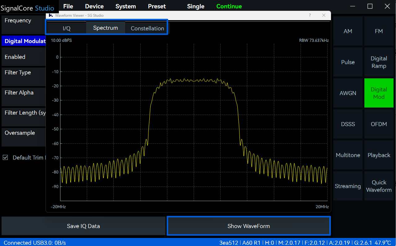
4. Click "Show WaveForm" to view the I/Q time-domain waveform, frequency-domain
spectrum, and constellation diagram.
Figure 6 Display waveform previews in digital modulation mode
5. Set the carrier "Frequency" to 1 GHz and "Power" to -20 dBm, then enable the RF output
switch;
6. The instrument outputs a BPSK digitally modulated signal with a center frequency of 1 GHz,
a peak power of -20 dBm, and a symbol rate of 10 MHz.
7
5.8 DSSS
Using a DSSS (Direct Sequence Spread Spectrum) signal with a carrier frequency of 1 GHz,
power level of -20 dBm, symbol rate of 300 kHz, BPSK modulation, and spreading code order
of 6 as an example:
Parameter Description
Table 19 DSSS Parameter Description
DSSS
Symbol Rate Number of symbols transmitted per second in the raw data
Constraint: Symbol rate ≤ Sampling rate / (Oversampling * (2^PN – 1))
Filter Type Rectangular, Raised Cosine, Root Raised Cosine, Gaussian, Half-Sine
| Filter Type | Rectangular, Raised Cosine, Root Raised Cosine, Gaussian, Half-Sine | |
|---|---|---|
| Filter Alpha | Specify the roll-off factor for the filter. | |
| Raised Cosine / Root Raised Cosine: [0.025,1]; Gaussian: [0.15,2.5] | ||
| Filter Length | Number of taps (order) for the filter. A greater length results in a filtering | |
| effect closer to the ideal, but at the cost of higher computational | ||
| complexity. Range: Even integers in [2, 400/OverSample]. | ||
| Oversample | Number of sample points per chip period. A higher oversampling rate | |
| results in a larger data volume and better signal quality. | ||
| Range: [4,32], must be an even number. | ||
| Sequence Seed | Initial value used to generate the pseudo-random sequence, ensuring | |
| that the generated sequence can be reproduced each time. | ||
| Modulation Type | Currently, only BPSK modulation is supported. | |
| Code | Order of the spreading code, range [4,16] | |
| The higher the order, the longer the generated spreading code sequence | ||
| (length = 2^ n-1), resulting in higher spreading gain and stronger anti- | ||
| jamming and anti-interception capabilities. However, a higher order also | ||
| increases system computational complexity and implementation | ||
| difficulty. |
Filter Alpha Specify the roll-off factor for the filter.
Raised Cosine / Root Raised Cosine: [0.025,1]; Gaussian: [0.15,2.5]
Filter Length Number of taps (order) for the filter. A greater length results in a filtering
effect closer to the ideal, but at the cost of higher computational
complexity. Range: Even integers in [2, 400/OverSample].
Oversample Number of sample points per chip period. A higher oversampling rate
results in a larger data volume and better signal quality.
Range: [4,32], must be an even number.
Sequence Seed Initial value used to generate the pseudo-random sequence, ensuring
that the generated sequence can be reproduced each time.
Modulation Type Currently, only BPSK modulation is supported.
Code Order of the spreading code, range [4,16]
The higher the order, the longer the generated spreading code sequence
(length = 2^ n-1), resulting in higher spreading gain and stronger anti-
jamming and anti-interception capabilities. However, a higher order also
increases system computational complexity and implementation
difficulty.
Operating Procedure
1. In the mode selection area, click "DSSS". In the control area, set the "Code" to 6;
2. Set "Oversample" to 4, "Symbol Rate" to 300 kHz, and enable the DSSS function;
3. Set "Frequency" to 1 GHz, "Level" to -20 dBm, and enable the RF output;
4. The instrument outputs a DSSS signal with a carrier frequency of 1 GHz, a peak power of -
20 dBm, a symbol rate of 300 kHz, BPSK modulation, and a spreading code length of 6.
8
5.9 OFDM
Parameter Description
Table 20 OFDM Parameter Description
OFDM
| Modulation Type | Set the modulation scheme used on each sub-carrier | ||
|---|---|---|---|
| Available options: BPSK, QPSK, 8PSK, 16PSK, QAM16, QAM64, QAM256 | |||
| FFT Size | Configure the total number of subcarriers for OFDM modulation | ||
| Range: 2 ^ n, where n ∈ {4, 5, 6, 7, 8, 9, 10, 11} |
Modulation Type Set the modulation scheme used on each sub-carrier
Available options: BPSK, QPSK, 8PSK, 16PSK, QAM16, QAM64, QAM256
FFT Size Configure the total number of subcarriers for OFDM modulation
Range: 2 ^ n, where n ∈ {4, 5, 6, 7, 8, 9, 10, 11}
Sample Rate Waveform Sampling Rate
| Carrier Spacing | Displays the frequency interval between two adjacent sub-carriers | ||
|---|---|---|---|
| under the current configuration. | |||
| Frequency Interval = Sample Rate / FFT Size. |
Carrier Spacing Displays the frequency interval between two adjacent sub-carriers
under the current configuration.
Frequency Interval = Sample Rate / FFT Size.
Symbol Count Set the number of OFDM symbols per burst.
Range: [2,16384].
Guard Band
Set the number of low-frequency edge guard sub-carriers. These are
not used for data transmission and serve as guard bands.
Carriers (Left)
Guard Band
Set the number of high-frequency edge guard sub-carriers. These are
not used for data transmission and serve as guard bands.
Carriers (Right)
Guard Interval (%) Set the Cyclic Prefix length as a percentage of the entire OFDM
symbol. This provides protection against multipath interference.
Null DC Enable: Disable the DC subcarrier (DC nulling is recommended)
Disable: Enable the DC subcarrier.
Windowed Whether a window function should be applied to the time-domain
waveform of the OFDM symbols to mitigate spectral leakage.
Window Length (%) Set the percentage of the windowing function applied to both ends
(bilateral) of the OFDM symbol. This value represents the total length of
the window function as a percentage of one OFDM symbol's duration.
The window function applies symmetrically to the leading and trailing
edges of the symbol.
Setting range: 0% to 100%, default: 50% (25% on each side).
Operating Procedure
Using the output of an OFDM signal closely matching the IEEE 802.11a standard as an example,
the configuration steps are as follows:
1. In the mode selection area, choose "OFDM";
2. Set "Modulation Type" to BPSK, "FFT Size" to 64, "Sample Rate" to 20 MHz, "Guard Band
Carriers (Left)" to 6, "Guard Band Carriers (Right)" to 5, and "Guard Interval (%)" to 25%. Leave
the remaining parameters at their default values, then enable the OFDM signal mode to
activate the current configuration;
9
3. Click "Save IQ Data" to save the current OFDM baseband signal in .wav format to the default
folder "SignalCore Studio/data";
4. Set the carrier "Frequency" to 5.18 GHz and "Level" to -10 dBm. Enable the RF output;
5. After completing the above settings, the instrument will output an OFDM signal with
characteristics approximating those of the IEEE 802.11a standard.
5.10 Multitone
Parameter Description
Table 21 Multitone Parameter Description
Multitone
| Tone Phase | Sets the initial phase generation method for each tone. Options | ||
|---|---|---|---|
| include Fixed, Random, or Parabolic. Different phase modes affect | |||
| the crest factor and dynamic range of the multitone signal. | |||
| Phase Random Seed | Provides the initial seed value for the pseudo-random number | ||
| generator used in "Random" phase mode. | |||
| Tone Count | Sets the number of discrete tones to be generated. | Sets the number of discrete tones to be generated. | |
| Frequency Spacing | Sets the frequency spacing between adjacent discrete tones. (Tone Count - 1) * Frequency Spacing ≤ 100 MHz. | ||
| Discrete Tone Mode | On: Configures the discrete tones in the multitone signal to be evenly | ||
| spaced. | |||
| Off: Allows in-band notch filtering (notching) of the multitone signal | |||
| by configuring the notch bandwidth. |
Tone Phase Sets the initial phase generation method for each tone. Options
include Fixed, Random, or Parabolic. Different phase modes affect
the crest factor and dynamic range of the multitone signal.
Phase Random Seed Provides the initial seed value for the pseudo-random number
generator used in "Random" phase mode.
Tone Count Sets the number of discrete tones to be generated.
Frequency Spacing Sets the frequency spacing between adjacent discrete tones.
(Tone Count - 1) * Frequency Spacing ≤ 100 MHz.
Discrete Tone Mode On: Configures the discrete tones in the multitone signal to be evenly
spaced.
Off: Allows in-band notch filtering (notching) of the multitone signal
by configuring the notch bandwidth.
Notch Width Sets the bandwidth of the notch filter.
Discrete tones within the notch range will be disabled.
| Frequency Offset | Displays the frequency offset of each discrete tone relative to the RF | ||
|---|---|---|---|
| center frequency. |
Frequency Offset Displays the frequency offset of each discrete tone relative to the RF
center frequency.
Enabled Independently enables or disables a specific indexed tone.
Operating Procedure
The following example demonstrates how to generate a multitone signal containing 5 discrete
tones, with a spacing of 2 MHz between each tone and a center frequency of 2.44 GHz.
1. Select "Multitone" in the mode selection area;
2. Set "Tone Count " to 5, set "Frequency Spacing" to 2 MHz, and enable Multitone mode;
3. Set the carrier "Frequency" to 2.44 GHz and "Level" to -10 dBm, then enable the RF output
switch;
4. After completing the above settings, the instrument will output the corresponding
multitone signal. The discrete tones will be distributed around the center frequency with a
spacing of 2 MHz.
10
5.11 Playback
The Playback mode, also known as the arbitrary file output function, supports the playback
of .wav waveform files, providing users with a highly flexible test signal generation solution.
This function adopts a preloaded storage mechanism to achieve high-performance signal
output. The software first loads the IQ waveform data into the instrument’s internal memory,
and the instrument directly plays back the preloaded data during operation. By avoiding real-
time transmission bandwidth limitations, the system ensures stable output of various complex
waveforms at the maximum analog bandwidth.
Parameter Description
Table 22 Playback Parameter Description
Playback
| Sample Rate | Sets the sampling rate of the arbitrary waveform. Maximum | ||
|---|---|---|---|
| supported: 125 MHz. It is recommended to match the original | |||
| waveform's sampling rate to avoid distortion. | |||
| Auto Scale | Enabled: The system automatically adjusts the amplitude of I/Q | ||
| waveform data so that the maximum sample value maps to full-scale | |||
| output. | |||
| Disabled: The waveform is output according to the set I/Q scaling | |||
| ratio. | |||
| I/Q Ratio (%) | When auto scaling is disabled, this ratio scales the amplitude of I and | ||
| Q data. 100% means no scaling. Adjustable range: 1% to 100%. | |||
| Period | Displays the total number of samples in the loaded waveform file. | ||
| If the user sets a number of points greater than the original, zeros are | |||
| automatically appended at the waveform tail. | |||
| Sample Offset | Sets the starting playback point within the arbitrary waveform file | ||
| Samples To Use | Number of samples actually used for output, starting from the point | ||
| offset. | |||
| Load | Loads waveform files in .wav format. File size must not exceed 125 | ||
| MB. | |||
| Unload File | Clears the currently loaded file, resetting related file parameters to | ||
| "N/A" or 0. | |||
| File Name | Displays the name of the loaded file. "N/A" indicates no file is loaded. | Displays the name of the loaded file. "N/A" indicates no file is loaded. | |
| Samples In File | Total I/Q sample pairs contained in the file. Determined by file size | ||
| and format; automatically updated after loading. | |||
| Signal Length | Actual playback duration based on Used Points and Sampling Rate: | ||
| Signal Length = Samples To Use / Sample Rate. | |||
| Period Length | Original duration of the file's data: | ||
| Period Length = Samples In File / Sample Rate. |
Sample Rate Sets the sampling rate of the arbitrary waveform. Maximum
supported: 125 MHz. It is recommended to match the original
waveform's sampling rate to avoid distortion.
Auto Scale Enabled: The system automatically adjusts the amplitude of I/Q
waveform data so that the maximum sample value maps to full-scale
output.
Disabled: The waveform is output according to the set I/Q scaling
ratio.
I/Q Ratio (%) When auto scaling is disabled, this ratio scales the amplitude of I and
Q data. 100% means no scaling. Adjustable range: 1% to 100%.
Period Displays the total number of samples in the loaded waveform file.
If the user sets a number of points greater than the original, zeros are
automatically appended at the waveform tail.
Sample Offset Sets the starting playback point within the arbitrary waveform file
Samples To Use Number of samples actually used for output, starting from the point
offset.
Load Loads waveform files in .wav format. File size must not exceed 125
MB.
Unload File Clears the currently loaded file, resetting related file parameters to
"N/A" or 0.
File Name Displays the name of the loaded file. "N/A" indicates no file is loaded.
Samples In File Total I/Q sample pairs contained in the file. Determined by file size
and format; automatically updated after loading.
Signal Length Actual playback duration based on Used Points and Sampling Rate:
Signal Length = Samples To Use / Sample Rate.
Period Length Original duration of the file's data:
Period Length = Samples In File / Sample Rate.
11
Operating Procedure
Using the output of an externally generated .wav IQ waveform file as an example, the operating
procedure is as follows:
1. Use signal editing software or other tools to generate a complex baseband signal with a
sample rate of 10 MHz, save it in .wav format with a file size not exceeding 125 MB (for
example, QPSK_signal.wav), and store the file in the ../data folder;
2. Click "Playback" in the mode selection area to enter the arbitrary file playback interface,
then click "Load";
3. In the pop-up file selection window, select the QPSK_signal.wav file in the data folder and
click "Open" to complete the loading process;
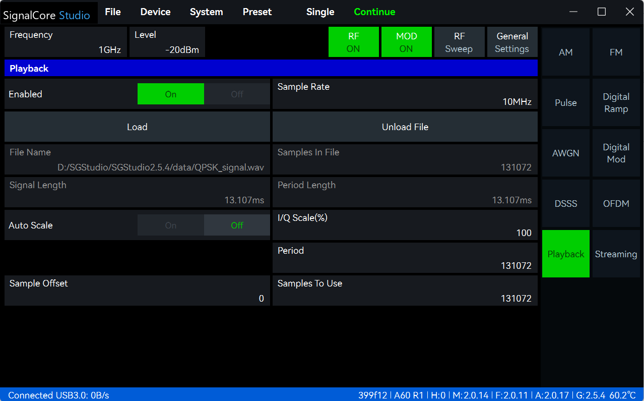
4. After the file is successfully loaded, the interface will display the total number of samples
and the corresponding playback duration. Set the "Sample Rate" to 10 MHz, while the
remaining parameters can be adjusted according to actual requirements (in this example,
all other parameters remain at their default settings), then enable the playback function;
5. Set the carrier "Frequency" to 1 GHz and the "Level" to -20 dBm, then enable the RF output
switch;
6. The signal generator will modulate the baseband IQ data from the loaded .wav file onto a 1
GHz carrier and output the RF signal from the RF port with a peak power of -20 dBm.
Figure 7 Playback mode
12
5.12 Streaming
Streaming mode is a mode that continuously outputs one or more WAV-format complex
baseband waveform files as RF signals. Data is loaded and transmitted in real time from an
external file system, enabling large-capacity and highly continuous signal output.
Parameter Description
Table 23 Streaming Mode Parameter Description
Streaming
| Sample Rate | Set the sampling rate of the waveforms in the file list, with a | ||
|---|---|---|---|
| maximum supported rate of 62.5 MHz. It is recommended to match | |||
| the original sampling rate of the signal to avoid distortion. No | |||
| resampling is performed when the sampling rates are inconsistent. | |||
| Load Files | Add waveform files to the file list for playback. Currently, only WAV | ||
| format is supported. |
Sample Rate Set the sampling rate of the waveforms in the file list, with a
maximum supported rate of 62.5 MHz. It is recommended to match
the original sampling rate of the signal to avoid distortion. No
resampling is performed when the sampling rates are inconsistent.
Load Files Add waveform files to the file list for playback. Currently, only WAV
format is supported.
Unload Files Remove all waveform files from the file list.
Remove File Remove the selected waveform file from the file list.
Operating Procedure
1. Use signal editing software to generate multiple .wav format complex baseband waveforms
(such as signal1.wav, signal2.wav, etc.) with a sampling rate of 10 MHz, and save these files
to the /data folder under the software directory;
2. Click "Streaming" in the mode selection area to enter the stream mode interface. Click "Load
Files", select the signal1.wav file in the pop-up file selection window, and click "Open" to
complete the loading process. To add multiple files, repeatedly click "Load Files" and select
additional .wav files in sequence (such as signal2.wav, signal3.wav, etc.);
3. After the files are successfully loaded, the interface will display the number of files, total
sample points, and total duration in the file list. Set the "Sample Rate" to 10 MHz. Other
parameters can be adjusted according to actual requirements (in this example, all other
parameters remain at their default settings), then enable the stream mode function;
4. Set the carrier "Frequency" to 1 GHz and the "Level" to -20 dBm, then enable the "RF" switch;
5. The instrument will then modulate and output the loaded waveform files, continuously
playing them in a loop. The playback progress will be displayed in real time in the stream
mode interface.
13
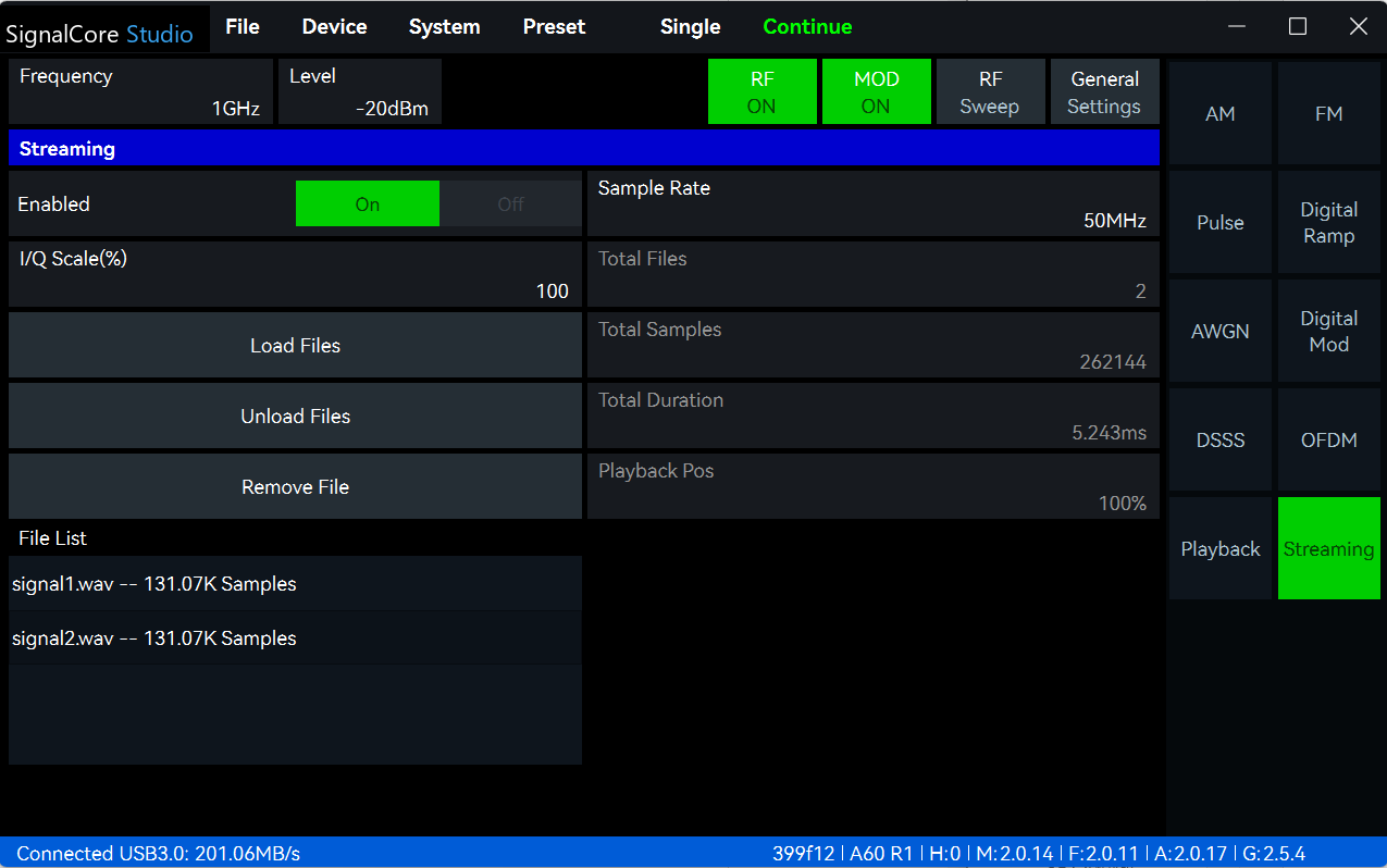
Figure 8 Streaming mode
5.13 Quick Waveform
In quick waveform mode, some preloaded waveform files in .wav format are available. You can
directly select the desired waveform and output it quickly.
Parameter Description
Table 24 Quick Waveform Parameter Description
Quick Waveform
| Sample Rate | Once the file is loaded successfully, the native sample rate of the | ||
|---|---|---|---|
| current file is displayed automatically. The user can further modify this | |||
| value as needed, up to a maximum of 125 MHz. | |||
| Load File | Click to select the WAV file from the file list and load it into the | ||
| instrument's internal memory. Only after successful loading can the | |||
| Quick Waveform Mode be enabled. | |||
| Auto Scale | Enabled: The system automatically adjusts the amplitude of I/Q | ||
| waveform data so that the maximum sample value maps to full-scale | |||
| output. | |||
| Disabled: The waveform is output according to the set I/Q scaling ratio. | |||
| I/Q Ratio (%) | When auto scaling is disabled, this ratio scales the amplitude of I and Q | ||
| data. 100% means no scaling. Adjustable range: 1% to 100%. | |||
| Period | Displays the total number of samples in the loaded waveform file. | ||
| If the user sets a number of points greater than the original, zeros are | |||
| automatically appended at the waveform tail. | |||
| Samples To Use | Number of samples actually used for output, starting from the sample | ||
| offset. |
Sample Rate Once the file is loaded successfully, the native sample rate of the
current file is displayed automatically. The user can further modify this
value as needed, up to a maximum of 125 MHz.
Load File Click to select the WAV file from the file list and load it into the
instrument's internal memory. Only after successful loading can the
Quick Waveform Mode be enabled.
Auto Scale Enabled: The system automatically adjusts the amplitude of I/Q
waveform data so that the maximum sample value maps to full-scale
output.
Disabled: The waveform is output according to the set I/Q scaling ratio.
I/Q Ratio (%) When auto scaling is disabled, this ratio scales the amplitude of I and Q
data. 100% means no scaling. Adjustable range: 1% to 100%.
Period Displays the total number of samples in the loaded waveform file.
If the user sets a number of points greater than the original, zeros are
automatically appended at the waveform tail.
Samples To Use Number of samples actually used for output, starting from the sample
offset.
14
| Sample Offset | Set the starting sample point position for waveform output. | ||
|---|---|---|---|
| The system will start reading waveform data from this offset position | |||
| for output. | |||
| File Name | Display the name of the currently pre-loaded waveform file. | ||
| Samples In File | Total I/Q sample pairs contained in the file. Determined by file size and | ||
| format; automatically updated after loading. | |||
| Signal Length | Actual playback duration based on Used Points and Sampling Rate: | ||
| Signal Length = Samples To Use / Sample Rate. |
Sample Offset Set the starting sample point position for waveform output.
The system will start reading waveform data from this offset position
for output.
File Name Display the name of the currently pre-loaded waveform file.
Samples In File Total I/Q sample pairs contained in the file. Determined by file size and
format; automatically updated after loading.
Signal Length Actual playback duration based on Used Points and Sampling Rate:
Signal Length = Samples To Use / Sample Rate.
Operating Procedure
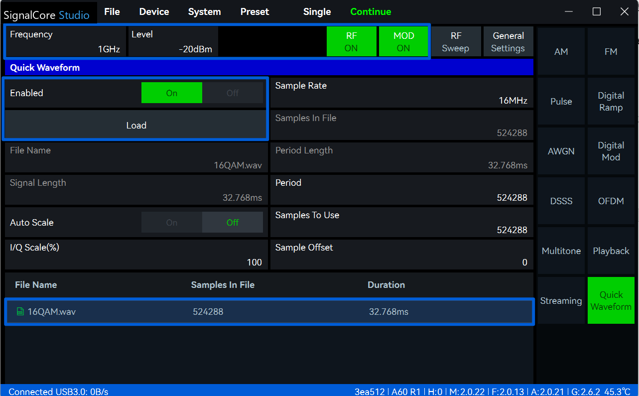
The following steps use the instrument’s preset 16QAM signal as an example to introduce the
basic operation of Quick Waveform mode.
1. Select "Quick Waveform" in the mode selection area.
2. Select "16QAM.wav" from the file list and click "Load Files" to load the selected waveform
into the instrument’s internal memory.
3. Once the file is loaded successfully, the software will automatically parse and display
the Sample Rate, total sample points, and signal length of the current file. Adjust the
corresponding parameters according to the test requirements, and then enable Quick
Waveform mode.
4. Set the Carrier Frequency to 1 GHz and the Level to -20 dBm, then enable the RF switch.
5. After completing the above settings, the instrument will output the 16QAM Quick
Waveform signal at a carrier frequency of 1 GHz and a peak power of -20 dBm.
Figure 9 Play the 16QAM Fast Waveform signal.
15
6. Software and Firmware Update
This section describes how to update the instrument’s software, FPGA, MCU, and Bus
versions.
6.1 Version Requirements
1. Refer to the viewing instrument information section to check the software and firmware
versions;
2. For all instruments, ensure that the GUI version is 2.5.4 or above;
3. If the software indicates that the update cannot be performed, please contact official
technical support.
6.2 Parameter Description
Note: Displays the current and target versions of the software, FPGA, MCU, and Bus;
Update Content: Provides detailed information about the changes in the target version;
Update Notification: Sets whether to automatically pop up an update notification window
when a new version is detected;
Update Method: The update methods are described in the table below.
Table 25 Update Method Description
Update Method Description
Online Automatically connects to the remote server to download and
install the latest software and firmware versions.
Local Manually loads an update package from a USB drive or local
storage for installation.
6.3 Online Update
1. Click "System" -> "Update" to enter the update interface;
2. Check the "Update Notification" checkbox. When the device is connected to the Internet,
the software automatically displays the Update window if a new version is detected during
startup or operation;
3. Set the "Update Method" to Online. The system will then start downloading the update
package, and the "Update" button will be temporarily disabled. After the package is
successfully downloaded and parsed, detailed release notes will be displayed in the
window, and the "Update" button will become enabled;
16
4. Carefully compare the information between the current version and the target version, and
review the new features and fix list. Once confirmed, click the “Update” button in the lower-
right corner;
5. After clicking, the software will automatically exit and enter the upgrade process. Please
keep the update window open until the progress bar completes and the software
automatically restarts and returns to the main interface.
17
18