1Start With the Load
A pulse generator is only as good as the match between its output stage and what it drives. So the first question is not "how many volts" but "what does the load look like." Loads fall into two families that place very different demands on the pulser.
A resistive load draws current in proportion to voltage, steady for the duration of the flat top, set directly by Ohm's law. A capacitive load draws current only while the voltage is changing, and that current is set by how fast you change it: I = C times dV/dt. The faster the edge and the larger the capacitance, the more peak current the output stage must deliver, even though the steady-state current at the flat top is near zero.
This is why capacitance, not voltage alone, sets the current demand for fast pulsing. A Pockels cell, a deflection plate, an extraction grid, or a length of coaxial cable all present capacitance. Drive a 100 pF load to 5 kV in 25 ns and the edge demands about 20 A of peak current (100 pF × 5,000 V / 25 ns), all of it to charge and discharge the capacitor.
The coax between the pulser and the load is part of the load. Common 50 ohm cable runs near 100 pF per meter, so a few meters can rival the capacitance of the device itself. Keep the run short, and include the cable when you total the capacitance the output stage must charge.
For a deeper treatment of charging a reactive load and keeping a fast edge clean into capacitance, see the companion note on pulsing capacitive loads. With the load capacitance known, each specification that follows can be checked against a number.
2Voltage Range and Bipolar Offset
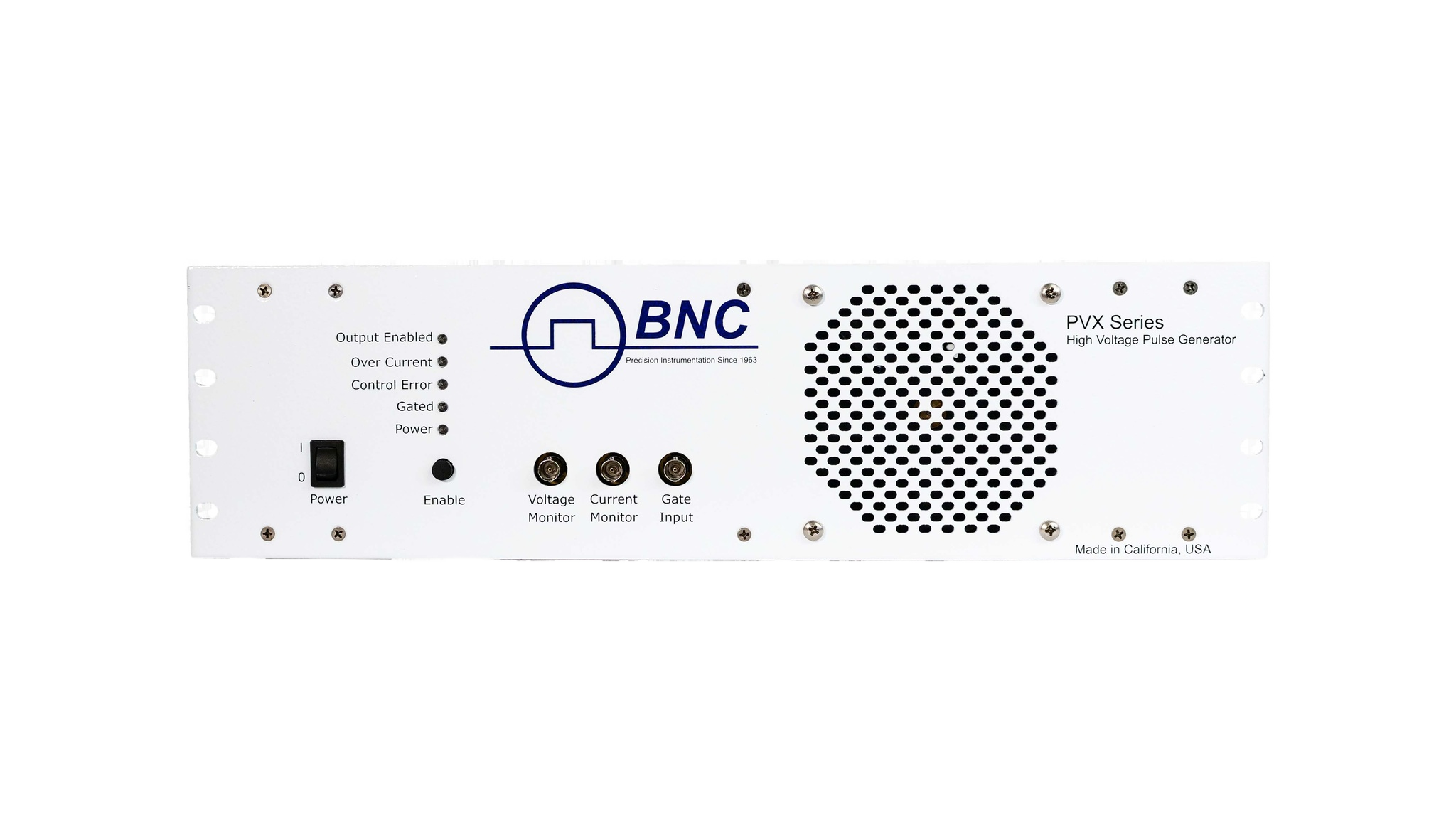
The voltage specification of a pulser is two numbers, not one. The PVX models and the PVM-4210 use a half-bridge output stage (Figure 1): an upper switch ties the output to a high rail (VHigh) and a lower switch ties it to a low rail (VLow). The output node sits between them, and the two switches operate in complement, so the output swings between VLow and VHigh rather than switching a single rail on and off.
That architecture is what gives a pulser its flexibility. Set VLow to ground and VHigh positive and you get a conventional unipolar positive pulse. Set VHigh positive and VLow negative and the output swings through zero into both polarities, a true bipolar swing. Many applications need it: bias networks driven above and below a reference, electro-optic cells that respond to field direction, and grids that require an active reset to a negative level rather than a passive decay.
When you read a model's voltage line, note whether it is a single magnitude, a plus-or-minus range, or a pair of supply inputs, because each places different limits on the levels. On the PVX-4110, PVX-4130, PVX-4141 and PVX-4151, VHigh and VLow are user-supplied DC inputs: each can sit anywhere within the model's rating (±10,000 V on the PVX-4110), provided VHigh is above VLow by no more than that rating. The PVX-4000-2kV sets its positive and negative levels from internal supplies, through the front panel or the computer interface, within a shared budget: V+ plus |V−| may not exceed 2,000 V. The PVM-1001 switches a single external high-voltage input and comes as separate positive (PVM-1001-P, 0 to +950 V) and negative (PVM-1001-N, 0 to −950 V) models. The PVM-4210 has one positive and one negative channel, each set from 0 to 950 V.
3Rise and Fall Time vs Your Timing Budget
Rise time and fall time set how quickly the output transitions between levels, and they matter for two reasons. First, they define the sharpness of the event: a Pockels cell that gates a laser pulse needs an edge faster than the optical window you want to open. Second, the edge speed drives the peak current into a capacitive load, as Section 1 showed, so a faster edge is not free.
Read the edge specification against your timing budget. If the experiment needs a 100 ns gate with 10 ns of margin at each end, an edge well under 10 ns leaves room; an edge of 60 ns does not. Where the amplitude is low and the transition must be as fast as possible, the 765-HV pulse generator delivers rise and fall times under 630 ps (10 to 90 percent) at up to 50 Vpp into 50 ohm. The PVM-1001 reaches 8 ns or less (PVM-1001-P, 200 V to 950 V) into a 50 ohm resistive load, with a slower fall of up to 50 ns at 450 V to 950 V. Into capacitive loads, the fastest edges in Section 10 are on the PVX-4141 and PVX-4151, at 25 ns or less into 50 pF. A slower edge is sometimes preferable: it lowers peak current, reduces ringing into a reactive load, and eases the average-power burden at high repetition rates.
If your timing margin is comfortable, a moderate edge draws less peak current and rings less into your cable, and can give a cleaner result than the fastest available part.
4Pulse Width and Duty Cycle
Pulse width is the time the output holds at the active level; duty cycle is the fraction of each period spent there. Together they connect the shape you want to the power the pulser must handle. A 1 microsecond pulse at 1 kHz is a 0.1% duty cycle and gentle on the output stage; the same width at 100 kHz is a 10% duty cycle and a very different thermal proposition.
Check three things. First, that the pulser can produce the minimum width you need without the edges merging, which sets a floor near the sum of the rise and fall times. Second, that it supports the maximum width or duty cycle you require: the PVX models and the PVM-4210 run from their minimum width to DC, while the PVM-1001 is limited to 10 µs and the PVX-2506 to 100 µs at up to 50 percent duty. Third, that width and repetition rate together stay inside the duty-cycle and average-power limits below. Pulse width, duty cycle, and average power are one connected budget.
5Droop and Flat-Top Fidelity
An ideal flat top holds a constant level for the full width of the pulse. A real one sags (Figure 2). Droop is that downward slope, and it comes from the finite energy stored in the output stage discharging into the load over the pulse duration. For a short pulse into a light load it is negligible. For a long pulse into a heavy or leaky load it can reach several percent, enough to matter when the flat-top level is the quantity your experiment depends on.
The same edges that carry the pulse can also carry overshoot, a brief excursion past the target level at the top of the rising edge, followed by ringing as the output settles. It is the interaction of the fast edge with the inductance and capacitance of the output and load. A clean flat-top specification accounts for all of it: the settling after overshoot, the droop across the hold, and the return to baseline. When flat-top accuracy drives your result, weigh droop and overshoot as heavily as the headline edge speed.
6Jitter
Jitter is the shot-to-shot variation in when the output edge arrives relative to the trigger. It is small, measured in picoseconds to nanoseconds, but it sets the floor on timing precision in any synchronized system. If a pulser gates a camera, fires a laser, or interleaves with other instruments on a shared timebase, jitter blurs the alignment between events.
For a single isolated pulse it rarely matters. For a system where many channels must land inside a tight window, or where many shots are averaged and must stack cleanly, low jitter is essential. Read the jitter figure against the timing window your experiment can tolerate, the same way you read edge speed against the gate width. A pulser with a fast edge but loose jitter can still miss a narrow coincidence window.
Among the models in Section 10, the PVX-4141 specifies jitter under 200 ps shot to shot; the PVX-4110, PVX-4130, PVX-4151 and PVM-4210 specify under 1 ns. Throughput delay, the fixed latency from gate to output, is a separate number (120 ns typical on the PVX-4141, 93 ns typical on the PVM-4210) and can be calibrated out; jitter cannot.
7Average-Power Limits
Every pulse deposits energy in the output stage, and the stage can only shed heat so fast. Average power, not peak voltage, is what usually limits sustained repetitive operation. It scales with energy per pulse times repetition rate, so a unit that drives a load comfortably at 1 kHz may overheat at 100 kHz even though every pulse is identical.
This is why a model's voltage rating and its maximum repetition rate are quoted together, and why the highest-voltage parts carry the lowest repetition-rate ceilings. Energy per pulse rises with the square of voltage and with load capacitance, so a 10 kV unit reaches its thermal limit at a rate about 44 times lower than a 1,500 V unit into the same load ((10,000 / 1,500)² ≈ 44). When you size a pulser for repetitive work, multiply through (energy per cycle times rate) and check the product against the maximum average power: 100 W on the PVX-4110, PVX-4130 and PVX-4141, 150 W on the PVX-4151, and 4 W per channel on the PVM-4210. The capacitive-load note covers this energy budget in more detail.
8Built-In Monitors
High-voltage, fast-edge signals are awkward to probe directly. A standard scope probe loads the node, and a high-voltage divider adds its own capacitance to the very thing you are measuring. That is why the PVX models provide built-in monitor outputs: a voltage monitor (V monitor) that reports a scaled replica of the output voltage, and a current monitor (I monitor) that reports the current the output stage is delivering.
The V monitor shows the flat-top level, droop, and overshoot without perturbing the output. The I monitor shows the peak charging current into a capacitive load, the quickest way to confirm that your edge speed and load capacitance are within the reach of the output stage. The PVX-4110 and PVX-4130 monitors scale 2000:1 (voltage, into 1 MΩ) and 10 A/V (current, into 50 Ω); the PVX-4141 and PVX-4151 scale 1000:1 and 10 A/V. The PVX-4000-2kV has a voltage monitor (1,000 V per 10 V) and a sync output and no current monitor, and the PVM-4210 and PVM-1001 modules have no monitor outputs.
9Single-Shot vs Repetitive Operation
The last axis is how often the pulse fires. Single-shot operation produces one pulse on command, with as much recovery time as needed before the next. Repetitive operation runs a continuous train at a fixed rate. The distinction matters because the limiting specification changes between the two modes.
In single-shot or low-rate work, peak performance dominates: you can use the full voltage and the fastest edge because there is time to cool between events. The PVX-2506, for instance, drives pulsed current-voltage tests where each measurement is a short burst with ample settling time. In high-rate work, average power dominates, as Section 7 described, and usable voltage or edge speed may have to back off to stay inside the thermal envelope. Some units add a burst mode that allows a short run above the continuous ceiling, useful when the experiment needs a brief fast train rather than indefinite operation. Decide which mode your application lives in before you compare numbers, because the same pulser can look very different in each.
10A Selection Starting Point
The table below maps DEI models against four numbers that narrow a search quickly: peak voltage, maximum repetition rate, edge speed, and jitter. Read it as a starting point, then return to the sections above to weigh droop, monitors, and the load match for the specific job. A row that clears your voltage and rate is a candidate until its flat-top fidelity and average-power envelope clear your application too.
| Model | Voltage | Max repetition rate | Rise time | Jitter (shot to shot) |
|---|---|---|---|---|
| PVX-4110 | ±10,000 V | single shot to 10 kHz | < 60 ns | < 1 ns |
| PVX-4130 | ±6,000 V | single shot to 10 kHz | < 60 ns | < 1 ns |
| PVX-4141 | ±3,500 V | single shot to 30 kHz (to 400 kHz at reduced load or voltage) | ≤ 25 ns | < 200 ps |
| PVX-4151 | ±1,500 V | single shot to 240 kHz (5 MHz burst) | < 25 ns | < 1 ns |
| PVX-4000-2kV / -EX | ±2,000 V, shared budget | 40 Hz to 30 kHz internal; external gate to 100 kHz (standard) or 600 kHz (EX) | ≤ 50 ns (500 V to 2,000 V) | not specified |
| PVM-4210 | +950 V and −950 V (1,900 V differential) | single shot to > 20 kHz (5 MHz burst) | ≤ 25 ns | < 1 ns |
| PVM-1001 | 0 to +950 V (-P) or 0 to −950 V (-N), 50 Ω load | to 1 MHz (5 MHz burst) | ≤ 8 ns rise (-P) / ≤ 50 ns fall, 450 V to 950 V | not specified |
| PVX-2506 | 0 to 50 V at 10 A | single shot to 50 kHz | < 200 ns | not specified |
Values are from the current published datasheets. Rise times are 10 to 90 percent into each model's reference load: 50 pF for the PVX-4110, PVX-4130, PVX-4141 and PVX-4151; 344 pF for the PVX-4000-2kV; a 50 Ω resistive load for the PVM-1001; and 5 Ω for the PVX-2506. Maximum rates at full voltage are limited by average power; Section 7 gives the ratings.
11Talk to an Engineer
The right pulser is the one whose weakest relevant specification still clears your application. That depends on details a table cannot capture: the exact load capacitance, the cable run, the timing window, the duty cycle, and how much droop or jitter your result can tolerate. Working those through with someone who knows the line is faster than reading datasheets alone.
For a quick question, an engineer can usually tell you in minutes whether a model fits or whether a different one in the line is the better match.
For help choosing, contact a BNC applications engineer at info@berkeleynucleonics.com or 800-234-7858.