Why these four numbers get confused
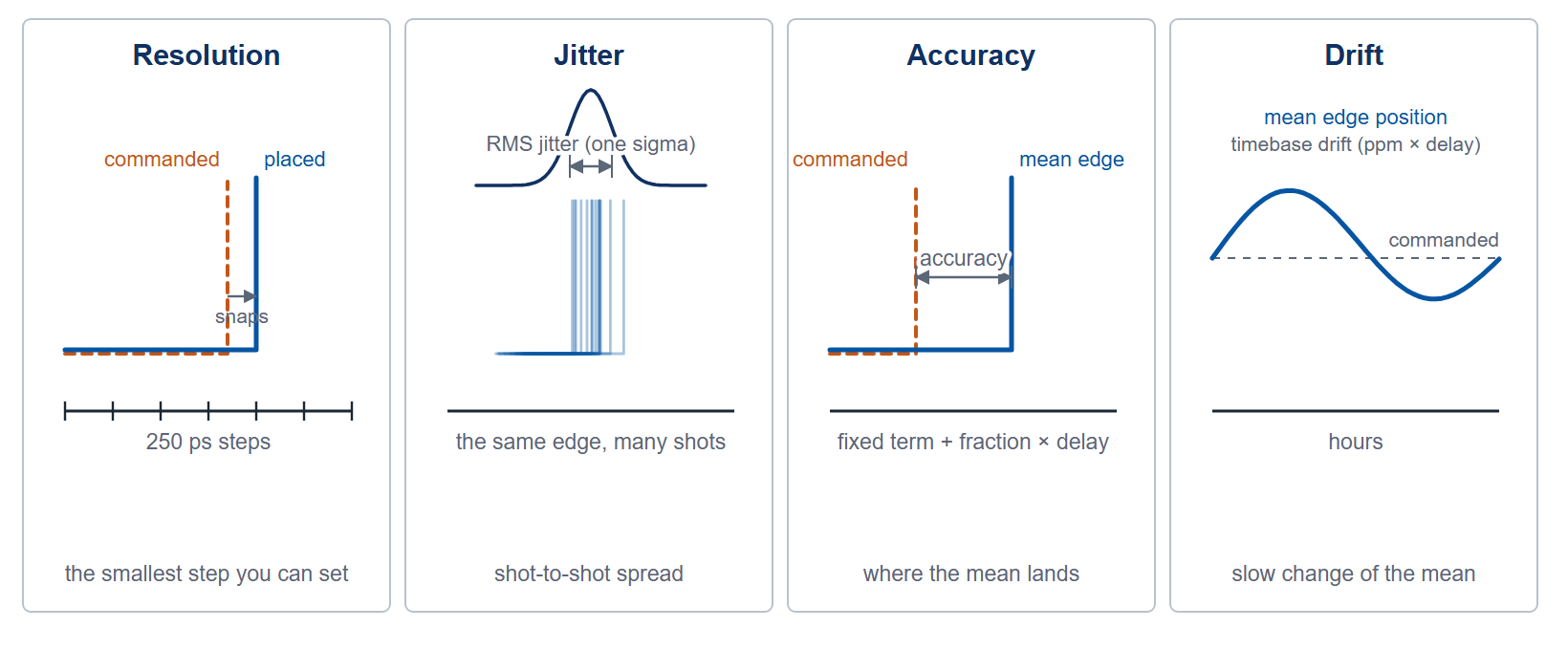
A datasheet line that reads "250 ps" can mean three different things depending on which column it is in. Resolution, jitter, and accuracy are separate properties of a timing instrument, and drift is a fourth that appears only indirectly, through the timebase rating. Choosing a delay generator on the wrong one of the four buys more instrument than the measurement needs, or less. Figure 1 sketches all four.
Delay resolution: the smallest step you can ask for
Resolution is the granularity of the delay setting. A 250 ps resolution means you can place an edge at 100.00 ns or 100.25 ns, but nothing between. It is a quantization limit, not an error. The Model 577 and Model 575 resolve to 250 ps. The Model 765 family steps in 10 ps. The Model 745T resolves 1 ps on channels A to D and 1.25 ns on its optional auxiliary channels E to H. Resolution sets the floor on how finely you can dial timing; it says nothing about how repeatable that timing is.
RMS jitter: shot-to-shot wobble
Jitter is the statistical spread of the actual edge around its commanded position, quoted as an RMS value. It is the number that limits how cleanly you can overlap two events or gate a fast detector. Low jitter is what lets a pulse generator define a coincidence window or a pump-probe interval.
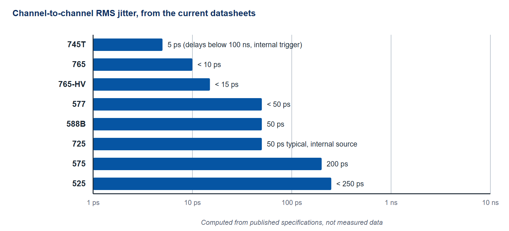
Jitter scales with where you measure it. Channel-to-channel jitter, the spread between two outputs of the same unit, is usually the tightest figure. Trigger-to-output jitter, measured from an external trigger, is larger because it includes the input comparator. The Model 588B specifies 50 ps RMS channel to channel. The Model 745T reaches about 5 ps RMS at delays below 100 ns. The Model 765 holds 4 ps RMS period jitter at 200 MHz and under 10 ps channel to channel, and the Model 577 stays under 50 ps channel to channel. By contrast a trigger input on the 575, 577 or 588B carries 800 ps RMS, so the path through the trigger input sets the budget, not the channel-to-channel figure. Figure 2 places the published channel-to-channel figures on one axis.
Timing accuracy: how close to the truth
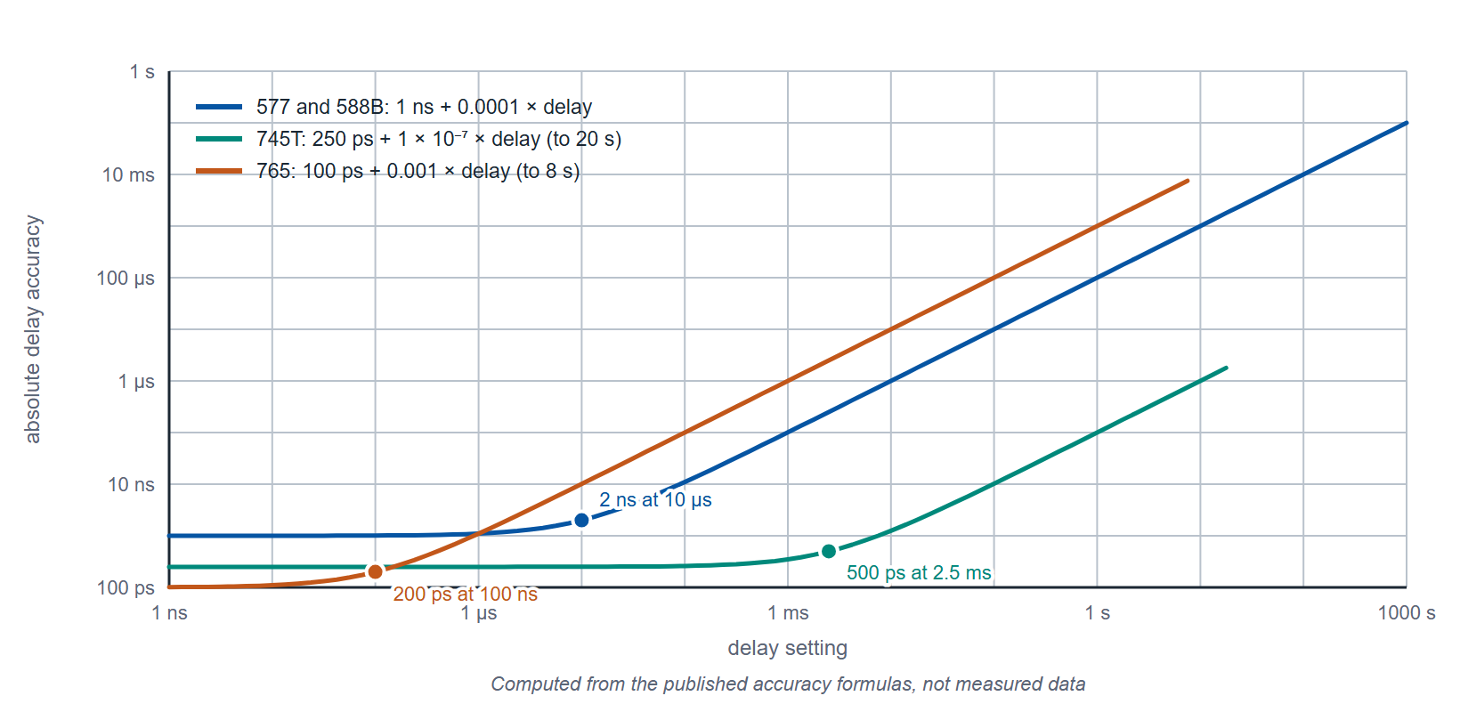
Accuracy is how far the mean edge position lies from the value you commanded. It is almost always written as a fixed term plus a fraction of the setpoint, for example 1 ns + 0.0001 times the delay. The fixed part dominates short delays; the proportional part, tied to the timebase, dominates long ones. The 575, 577 and 588B quote 1 ns + 0.0001 times the setpoint, so the two terms are equal at a 10 µs delay and the proportional term is ten times the fixed one at 100 µs. The 745T specifies 250 ps plus delay times ten to the minus seven, with a 0.5 ppm TCXO timebase as standard and a 0.05 ppm OCXO as an option. The 765 family quotes ±(0.1% + 100 ps) on delay and ±2 ppm on period. Accuracy and jitter together describe a distribution: accuracy is where the center lies, jitter is how wide it spreads. Figure 3 shows how the proportional term overtakes the fixed term as the delay setting grows.
Drift: the slow one
Drift is the change in timing over minutes to hours, driven mostly by temperature and crystal aging. It does not appear as a single spec line; it hides inside the oscillator rating. A 25 ppm oscillator, as in the Model 588B, will move more across a 20 degree swing than the 745T's 0.5 ppm timebase, or its 0.05 ppm option. For short experiments drift is irrelevant. For a synchronization system that runs all day, it can exceed jitter by orders of magnitude, which is why locking to an external 10 MHz reference matters. The 575, 577 and 765 family accept a 10 to 100 MHz external clock, the 588B 10 to 80 MHz in discrete steps, and the 745T a 10 MHz reference as standard.
How the models compare
| Model | Delay resolution | RMS jitter | Accuracy | Timebase |
|---|---|---|---|---|
| 525 | 4 ns | <50 ps (rate generator); <250 ps ch-to-ch | 5 ns + 0.0001 × delay | 50 MHz, 50 ppm (1 ppm option) |
| 575 | 250 ps | 200 ps (delay); 50 ps (rate generator) | 1 ns + 0.0001 × setpoint | 25 ppm |
| 577 | 250 ps | <50 ps ch-to-ch | 1 ns + 0.0001 × setpoint | 100 MHz PLL; 50 MHz, 50 ppm oscillator |
| 588B | 250 ps | 50 ps ch-to-ch | 1 ns + 0.0001 × delay | 200 MHz PLL; 50 MHz, 25 ppm oscillator |
| 725 | 10 ns | 50 ps typ / 200 ps max (internal source) | 0.001% typ, 0.01% max | internal clock, 1.5625 to 100 MHz |
| 745T | 1 ps (A to D); 1.25 ns (E to H) | ~5 ps below 100 ns delay; 25 ps + delay × 10⁻⁷ from an external trigger | <250 ps + delay × 10⁻⁷ | 0.5 ppm TCXO; 0.05 ppm OCXO option |
| 765 | 10 ps | 4 ps period (200 MHz); <10 ps ch-to-ch | ±(0.1% + 100 ps) delay; ±2 ppm period | ±2 ppm |
| 765-HV | 10 ps | <15 ps period; <15 ps ch-to-ch | ±(0.1% + 100 ps) delay; ±2 ppm period | ±2 ppm |
Table 1. Values from the current datasheets. Jitter figures are RMS, with the datasheet's condition where it states one.
Reading the budget in practice
Add the relevant terms for your case, do not take the smallest number on the page. A pump-probe setup triggered externally inherits the trigger jitter, not the channel-to-channel figure. A long delay inherits the timebase term, not only the fixed accuracy. And a system that runs for hours inherits drift unless it is locked to a reference. The budget is the sum of the terms on the path in use.
A worked case: a Model 577 triggered externally, with one channel set to a 10 µs delay. The trigger input contributes 800 ps RMS of jitter and the channel-to-channel figure is under 50 ps RMS, so the window has to be designed around the 800 ps, not the 50 ps. The delay accuracy is 1 ns + 0.0001 × 10 µs = 2 ns, half of it from the timebase term. Running the same setup from the internal rate generator removes the 800 ps and leaves the 50 ps; the 2 ns stays.
Get help sizing the budget
Tell us the trigger source, the delays involved, and the runtime, and we will work the jitter and accuracy budget with you against the datasheet figures. Reach Berkeley Nucleonics at info@berkeleynucleonics.com or 800-234-7858, or browse the full Pulse & Delay Generators documentation.