LiDAR Testing
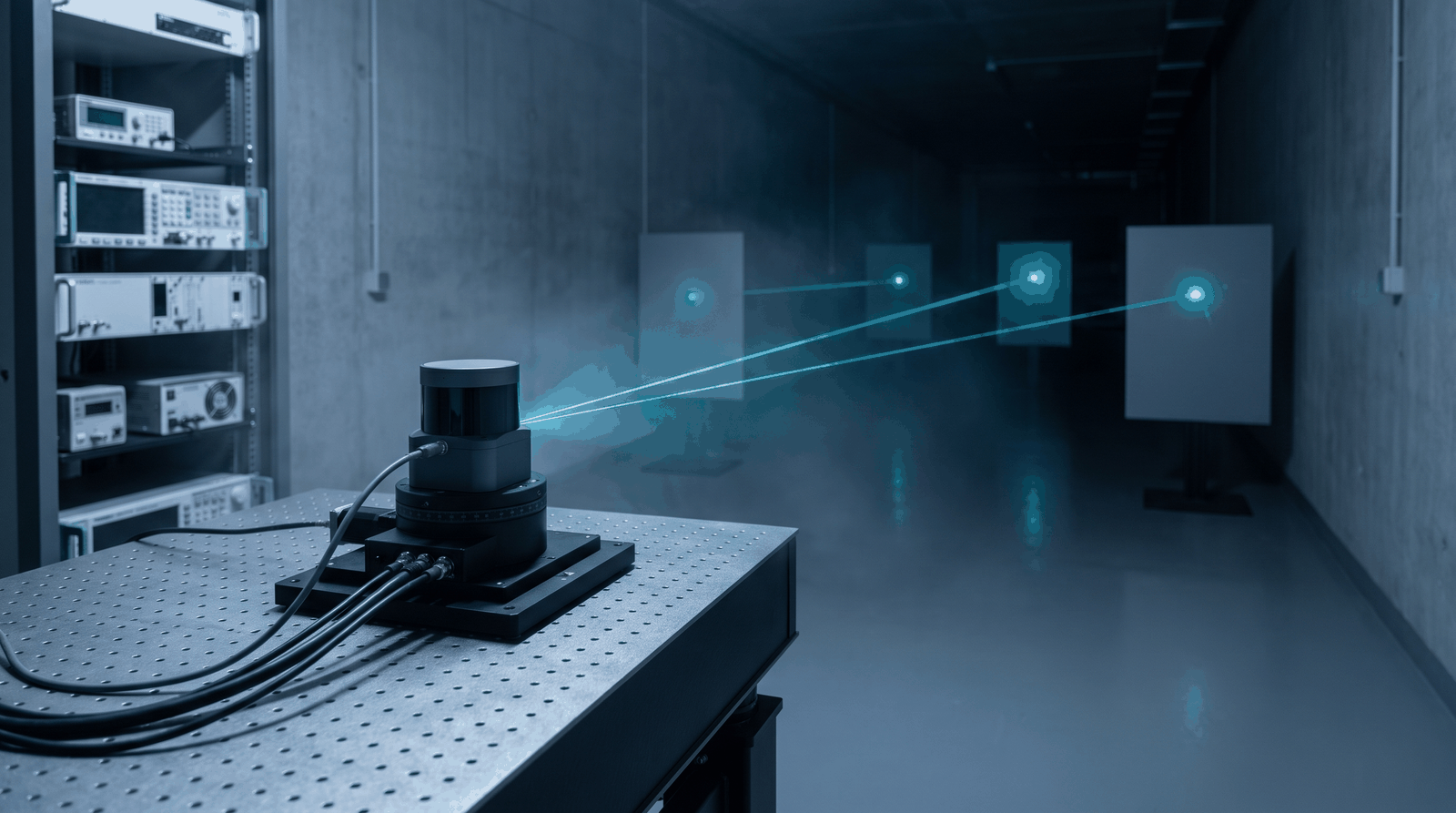
A LiDAR sensor measures range from the time between an emitted laser pulse and its reflection, t = 2R/c, so the bench that validates it has to produce those reflections at the times and amplitudes a real scene would. Scenario emulation means generating the full set of return pulses a sensor would see in a scene: near and far targets, faint and bright returns, multiple objects layered in a single field of view, each placed at the delay its range sets (Figure 1). The pulsed-laser-diode side of the problem is the mirror image: the bench drives the emitter itself and shapes the optical pulse the sensor sends out.
Both tasks share two requirements. The waveform has to be long, because a realistic scenario spans a wide time window and carries many distinct pulses. The timing has to be fine: 1 cm of range is 66.7 ps of round-trip time, and 1 mm is 6.7 ps. When a LiDAR unit uses several detector channels or several emitters, the bench feeds all of them at once and holds them to one timebase.
The challenge
Two limits set how much of a scene a waveform generator can reproduce. The first is memory depth. The return window for a 300 m maximum range is 2.0 µs long, which is 40,000 samples at 20 GS/s, so a record of 10,000 distinct return windows needs 400 Msamples. When a scenario does not fit in one record, it has to be shortened, looped or assembled from sequencer segments, and each of those changes what the sensor sees.
The second limit is timing. Each emulated return carries the timing uncertainty of the path that places it: trigger-to-output jitter when the sensor's emission triggers the generator, and channel-to-channel skew when returns or emitters are spread across several outputs. In range terms, 10 ps rms of timing jitter is 1.5 mm rms of range, so the bench's timing budget is set against the range resolution the sensor is specified to.
How the Model 686 solves it

The Berkeley Nucleonics Model 686 (Figure 2) samples at up to 20 GS/s with 14-bit vertical resolution. In True Arb mode at full rate, CH1 holds up to 9.6 Gsamples (CH1 and CH3 on the 4-channel models): 0.48 s of continuous waveform at 20 GS/s, or 240,000 of the 2.0 µs return windows above. The other channels are shorter, 1.17 Msamples on CH2 of the 2-channel models and 589 ksamples on CH2 and CH4 of the 4-channel models (58.5 µs and 29.45 µs at 20 GS/s), so the long scenario belongs on CH1 or CH3 and the short-memory channels suit repeating patterns such as emitter drive. The sequencer chains up to 16,384 entries for scenarios longer than one record.
The Model 686 timing figures each carry their own condition. Trigger In to output jitter is 0.29 × DAC clock period rms in True Arb mode, which is 14.5 ps rms at 20 GS/s (2.2 mm rms of range), and under 20 ps rms in AFG mode. Random jitter on a clock pattern is under 2 ps rms; it describes the output edges, not the trigger path. Channel-to-channel skew is adjustable over 0 to 1.63 µs with 100 fs resolution between CH1 and CH2 on the 2-channel models (between the CH1/CH2 and CH3/CH4 pairs on the 4-channel models), with ±(1% of setting + 20 ps) accuracy and under 20 ps initial skew. The sample period at 20 GS/s is 50 ps, or 7.5 mm of range: the time grid on which each return is placed in the record.
The trigger path also has latency. In True Arb mode the trigger-to-output delay is under 4,392 DAC clock periods plus 17.6 ns, which is under 237.2 ns at 20 GS/s, the round-trip time to a target 35.6 m away. Firing the sensor from a Model 686 marker output instead places the emission and the emulated returns on one waveform timeline; the remaining offset is the sensor's own fire latency, which is measured once on the bench.
When a bench needs more channels than one chassis provides, up to four Model 686 units synchronize over the dedicated sync bus (QSFP Sync In and Sync Out, RIDER-686-SYNC cable): four 4-channel units give 16 analog and 128 digital channels. Alignment between units is set during calibration rather than specified: measure the offset between units on the bench and remove it with the channel skew adjustment before calibrating the scene.
The single-ended models (686-2C-SE and 686-4C-SE) deliver up to 5 Vpp into 50 Ω, which drives pulsed-laser-diode test fixtures rated for that swing directly, without an external amplifier adding its own delay and distortion. True Arb rise and fall times are 50 ps or less (20% to 80%) and 70 ps or less (10% to 90%), at 1 Vpp single-ended. Where a fixture needs more than 5 Vpp, a Model 686 marker output triggers a Berkeley Nucleonics Model 765-HV pulse generator: up to 50 Vpp into 50 Ω (output limits −25 V to +25 V), rise time under 630 ps (10% to 90%) at up to 50 Vpp, and pulse width from 1 ns to the period minus 1 ns. Its trigger input accepts ±3.5 V into 50 Ω or ±10 V into 1 kΩ, and the 686 keeps the scenario timing.
Recommended configuration
For scenario emulation, put the longest scene on CH1 (or CH3 on a 4-channel model) of one Model 686 so it plays from a single record, and lock the 686 reference clock input (5 MHz to 500 MHz) to the bench master so the generator and the bench share one frequency reference. Fire the sensor from a marker output, or trigger the 686 from the sensor's emit signal and budget 14.5 ps rms of trigger jitter and up to 237.2 ns of trigger delay at 20 GS/s. Lay out the target returns on the 50 ps sample grid and use the 5 Vpp output to drive the detector test fixture directly.
For a multi-channel LiDAR system, add Model 686 units on the sync bus, up to four in all, so emitters and detectors share one timebase, and measure the unit-to-unit alignment once at setup. Where a fixture needs more than 5 Vpp, add a Model 765-HV for drive up to 50 Vpp and fire it from the 686. Build each scenario once in memory and reference every unit to the master clock, so each run plays the same scene against the same reference. Channel count (2 or 4) and output type (single-ended, 5 Vpp, or differential, 2.5 Vpp) are ordering choices.
Talk to an application engineer
Berkeley Nucleonics works with OEM sensor labs, defense electro-optical and infrared test groups, and LiDAR hardware teams to match the Model 686 and its pulse-generator pairing to a specific bench. Call 800-234-7858 or email info@berkeleynucleonics.com.
For a quick question, chat with an engineer at berkeleynucleonics.com.
Ask now → Chat with our assistant and get an answer in seconds.