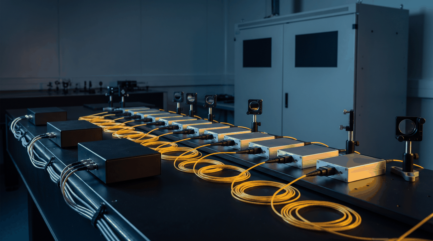
HEL / ICF Front-End Timing
A high-energy-laser or inertial-confinement-fusion front end shapes a low-power seed pulse before the amplifier chain. An electro-optic modulator carves the temporal shape, an acousto-optic modulator gates or picks pulses, and both are driven by electrical waveforms timed against the facility's master reference. The drive stage has two jobs against one clock: place the pulse at a known instant relative to every other beamline and diagnostic, and give it the shape that, after the gain saturation of the amplifiers, produces the shape wanted on target.
Both jobs have numbers. Light travels 0.30 mm per picosecond, so 10 ps of timing error between two beamlines is 3 mm of path at the target, and a multi-beam facility writes its beam-to-beam budget in tens of picoseconds. On the shape, a stored waveform has to resolve the fastest feature of the pulse and hold a low-intensity foot ahead of a high-intensity peak: a 30 ns shaped pulse at 50 ps per sample is 600 samples, and at 14 bits a foot at 1 percent of the peak is still represented by 164 of 16,384 levels.
The front-end timing stage
The conventional stage is a chain: a reference distribution unit, a trigger or delay generator, a shaping generator, and a driver amplifier for each modulator. Each element does its part well. A Digital Delay Generator places an edge with picosecond resolution, and a dedicated shaping generator holds a stored profile. The limit of the chain is the number of clock domains in it and the drift between them. Every unit that free-runs on its own oscillator carries its own aging and temperature drift, and every cable between units is a delay that moves with temperature. The stage holds its alignment more easily when timing and generation share one clock, which is what an arbitrary waveform generator disciplined to the facility reference provides.
How the Model 686 is used
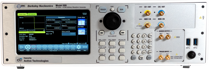
The Berkeley Nucleonics Model 686 takes the facility reference directly. The reference clock input accepts 5 to 500 MHz at 0.2 to 3.3 Vpp into 50 ohm, so a 10 MHz or 100 MHz house reference disciplines the instrument's 20 GS/s sample clock. Where the facility distributes a sample-rate clock instead, the external clock input accepts the sample rate divided by 8, 16, 32 or 64 at 0 to +10 dBm, which at 20 GS/s is 2.5 GHz, 1.25 GHz, 625 MHz or 312.5 MHz. Either way the output runs on the facility's timebase rather than on the internal reference, which on its own is accurate to 1 ppm (500 ppb with the optional 100 MHz oven-controlled oscillator).
The shot fiducial goes to the trigger input. Trigger-to-output jitter is under 20 ps rms in AFG mode and 0.29 sample clock periods in True Arb mode, which at 20 GS/s is 14.5 ps rms. The trigger input carries a programmable delay of 0 to 2,418 ps in 78 ps steps, and the trigger-to-output delay is bounded, under 205 ns in AFG mode and under 4,392 clock periods plus 17.6 ns in True Arb mode (237 ns at 20 GS/s), so it enters the facility delay table as a fixed term. Within one instrument the analog channels start within 20 ps of each other, and the skew between them is adjustable from 0 to 1.63 µs in 100 fs steps at an accuracy of 1 percent of the setting plus 20 ps. The 100 fs is the step size of that adjustment; the alignment a beamline can rely on is the accuracy term. Across separate instruments linked by the synchronization bus, alignment is measured at commissioning rather than taken from a specification.
The pre-shaped waveform of Figure 1 is a stored arbitrary waveform. The pre-compensation is computed by the facility from the measured gain of its amplifier chain and loaded as samples; the instrument plays it at 20 GS/s with 14-bit amplitude resolution and edges of 70 ps or less (10 to 90 percent at 1 Vpp). Waveform memory on channel 1 is 9.6 Gsamples, which is 0.48 s at full rate; channel 2 holds 1.17 Msamples, which is 58.5 µs, enough for a gate waveform or a diagnostic trigger but not for a long record. The sequencer holds up to 16,384 entries with loops, jumps and conditional branches, so a shot schedule is stepped through from memory rather than reloaded between shots.
Output amplitude is 5 Vpp into 50 ohm. As a sine that is 62.5 mW, or +18 dBm. A waveguide electro-optic modulator whose half-wave voltage lies within that swing is driven directly. An acousto-optic modulator that needs 1 W of RF at its carrier takes a 12 dB power amplifier after the generator, and the generator supplies the modulated carrier with the gate timing already in it. A free-space Pockels cell at kilovolts takes a high-voltage pulser such as the DEI PVM-4210 (two outputs to plus or minus 950 V, edges under 25 ns, widths from under 50 ns to DC), gated from a Model 686 marker or channel.
Recommended configuration
For a single beamline front end, a two-channel Model 686-2C-SE: channel 1 drives the electro-optic modulator with the stored pre-shaped waveform, channel 2 supplies the acousto-optic gate (carrier and envelope together) or a diagnostic trigger, the house 10 MHz or 100 MHz reference feeds the reference clock input, the shot fiducial feeds the trigger input, and the marker outputs trigger the streak camera or digitizer.
For a multi-beamline facility, a four-channel Model 686-4C-SE places four drives on one chassis, with the channels starting within 20 ps of each other and the pair-to-pair skew adjustable in 100 fs steps. Up to four instruments on the synchronization bus give 16 channels, with the alignment between chassis measured and entered in the facility delay table at commissioning.
Limitations. The instrument does not measure or model the amplifier chain; the pre-compensation is the facility's, and it changes when the chain does. The trigger jitter figures are relative to the trigger edge, so alignment to the facility clock is only as good as the reference and trigger distribution feeding the instrument. Channel 2 memory is 1.17 Msamples, so long records go on channel 1. Cross-unit alignment is not a published specification.
Talk to an application engineer
Berkeley Nucleonics can help you match a Model 686 configuration to your HEL or ICF front-end timing stage. Call 800-234-7858 or email info@berkeleynucleonics.com. Specifications: Model 686 datasheet.
For a quick question, chat with an engineer at berkeleynucleonics.com.
Ask now → Chat with our assistant and get an answer in seconds.