Phase Noise Measurement Basics

Every oscillator, synthesizer and clock carries a small random fluctuation in its phase. On a spectrum display it shows as noise skirts on either side of the carrier. In a receiver it mixes an adjacent-channel blocker into the wanted channel. In a digital link it rotates every symbol. In a data converter it becomes aperture jitter. One number, single-sideband phase noise, describes all four, and this note explains what the number means, how it is integrated into rms phase and time jitter, how the three measurement architectures differ, and how to read an analyzer's sensitivity table before trusting a plot. It is written for the design or test engineer who has to specify, measure or defend a phase noise figure, including one meeting the measurement for the first time.

1. What phase noise is

A real source does not produce a pure cosine. Its output is a carrier at frequency f₀ with a slowly varying amplitude error α(t) and a phase error φ(t). Phase noise is the frequency-domain description of φ(t). Figure 1 shows how it appears: the carrier line sits on a pedestal of noise that falls away with offset from the carrier, and discrete lines, the spurs, stand above the pedestal at fixed offsets.

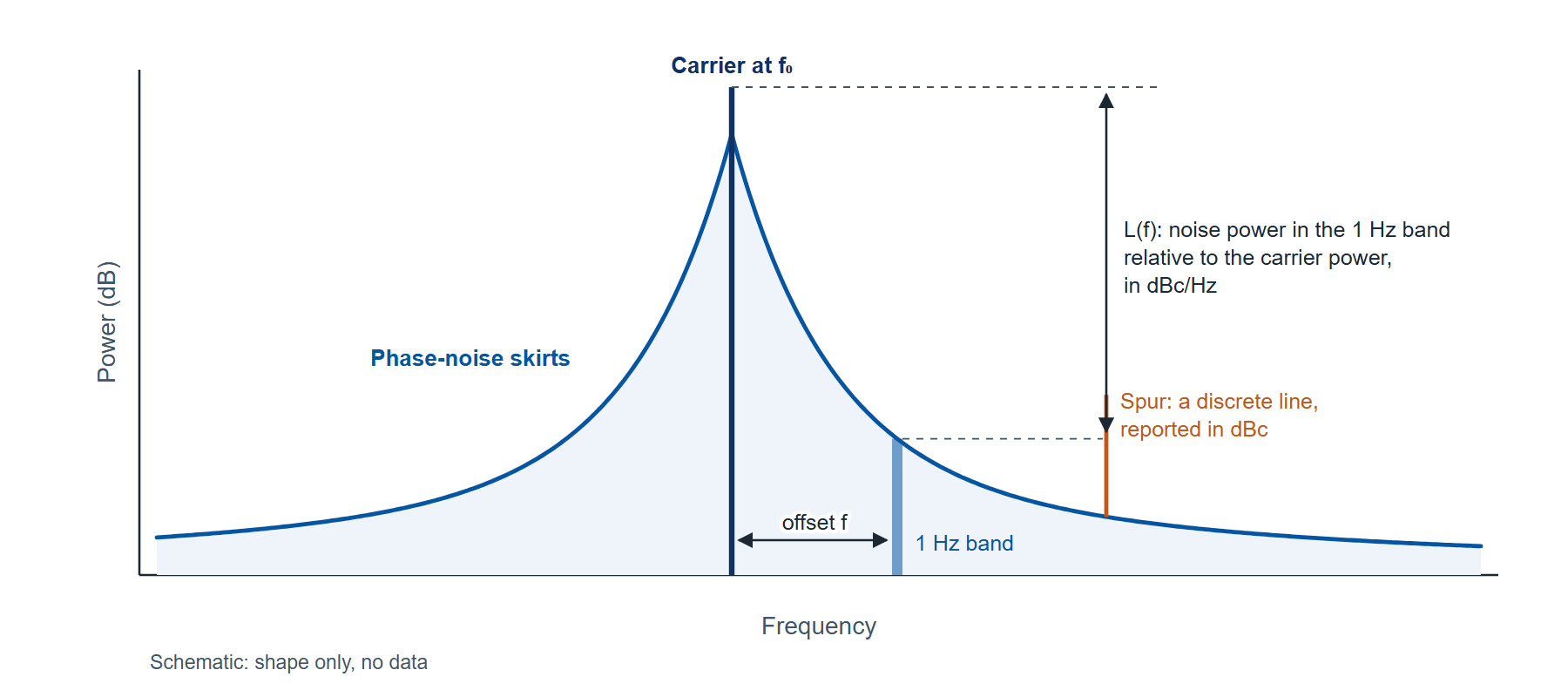
Figure 1. Schematic. A carrier with its phase-noise skirts and one spur. Single-sideband phase noise L(f) is the noise power in a 1 Hz bandwidth at offset f from the carrier, relative to the carrier power; a spur is a discrete line and is reported in dBc, not dBc/Hz. — PhotoFigure 1. **Figure 1.** Schematic. A carrier with its phase-noise skirts and one spur. Single-sideband phase noise L(f) is the noise power in a 1 Hz bandwidth at offset f from the carrier, relative to the carrier power; a spur is a discrete line and is reported in dBc, not dBc/Hz.

The quantity an analyzer reports is defined by IEEE Std 1139 as half the one-sided spectral density of the phase fluctuation:

L(f) = ½ S_φ(f)(1)

where S_φ(f) is the one-sided power spectral density of the phase fluctuation in rad²/Hz, f is the offset from the carrier in Hz, and L(f) is expressed in dBc/Hz as 10 log₁₀ of the ratio. A reading of −130 dBc/Hz at 1 kHz means that a 1 Hz band centered 1 kHz from the carrier holds 10⁻¹³ of the carrier power.

The definition settles two things a plot alone does not. It refers to phase, so amplitude noise is a separate quantity measured a different way. And it is a density, so a spur, which has a fixed power regardless of bandwidth, cannot be read off the same axis; a good analyzer lists spurs in dBc in a separate table.

Integrating the density over a band gives the rms phase error in that band, and dividing by the carrier's angular frequency converts it to time:

φ_rms² = 2 ∫_{f_L}^f_H L(f) df(2)

t_j = φ_rms / (2π f₀)(3)

where L(f) is taken as a linear ratio, not in dB; f_L and f_H are the integration limits in Hz (10 Hz to 1 MHz is a common reporting band; the right band is set by the application, as section 2 shows); φ_rms is in radians; and t_j is the rms time jitter in seconds for a carrier at f₀ Hz. The factor 2 restores both sidebands.

In practice the integral is evaluated on the plotted points, treating L(f) as a straight line in dB against log offset between neighbors. Section 5 works one through. An integrated phase quoted without its band is not a specification, because on most sources the integral depends strongly on where it starts.

The shape of the curve carries information about the source. Table 1 lists the regions a free-running or locked source shows, from the carrier outward. Inside a phase-locked loop's bandwidth the reference and the loop set the curve; outside it the oscillator's own noise takes over; and far out, the curve flattens onto a white phase floor set by the source's output stage and, in the measurement, by thermal noise.

**Table 1.**
Region (from the carrier outward)	Slope of L(f)	Usual cause
Random-walk frequency noise	−40 dB per decade	Environment: temperature, vibration, supply drift
Flicker frequency noise	−30 dB per decade	The resonator and the active device, up-converted
White frequency noise	−20 dB per decade	Thermal noise inside the oscillator loop
Flicker phase noise	−10 dB per decade	Amplifier and buffer 1/f noise
White phase noise (the floor)	0 dB per decade	Thermal noise of the output stage; in a measurement, the instrument floor
Spurs	Discrete lines	Supply ripple, reference leakage, fractional-N artifacts, coupling

2. Why the number matters, with one worked case each

A receiver. A local oscillator's phase noise is transferred onto every signal it mixes. A strong blocker at offset f from the wanted channel is spread by the LO's L(f) into the channel, a mechanism called reciprocal mixing. The noise it deposits is the blocker power plus L(f) plus 10 log₁₀ of the channel bandwidth. For a −30 dBm blocker 1 MHz away, an LO at −130 dBc/Hz at 1 MHz and a 1 MHz channel: −30 + (−130) + 60 = −100 dBm. A receiver with a 5 dB noise figure has a thermal floor in that channel of −174 + 60 + 5 = −109 dBm, so the LO, not the front end, sets the sensitivity in the presence of that blocker by 9 dB. The offsets that matter are the channel spacings of the system, which is why a receiver specification names L(f) at particular offsets rather than an integrated figure.

A digital link. A carrier-recovery loop tracks the phase noise inside its bandwidth; the noise outside it rotates every symbol by a random angle whose rms value is φ_rms from equation (2), integrated from the loop bandwidth outward. On a 64-QAM constellation the outer symbol at (7, 7) on its unit grid crosses its decision boundary at 6 when rotated by 7.7 degrees (cos(45° + θ) = 6 / (7√2) gives θ = 7.7°). An rms phase of 1 degree leaves that symbol a margin of 7.7 times its rms error; 2.5 degrees leaves 3 times. The band that matters here starts at the loop bandwidth, typically kilohertz, and ends at the symbol rate.

A sampling clock. For a converter clock the quantity is time jitter, equation (3). An rms phase of 0.01 degrees (1.75 × 10⁻⁴ rad) on a 1 GHz clock is 1.75 × 10⁻⁴ / (2π × 10⁹) = 28 fs. How that jitter limits a converter's signal-to-noise ratio is worked in the companion note on selecting a low-jitter clock source. The band that matters is set by the converter and the downstream processing, and again begins near the carrier.

Three applications, three different bands. The common thread is that each needs the curve, not a single number, and each needs it measured with an instrument whose own noise is known to be below it.

3. How phase noise is measured: three architectures

Figure 2 draws the three ways the measurement is made. Each works, and each has a limit that belongs to the architecture rather than to any particular instrument.

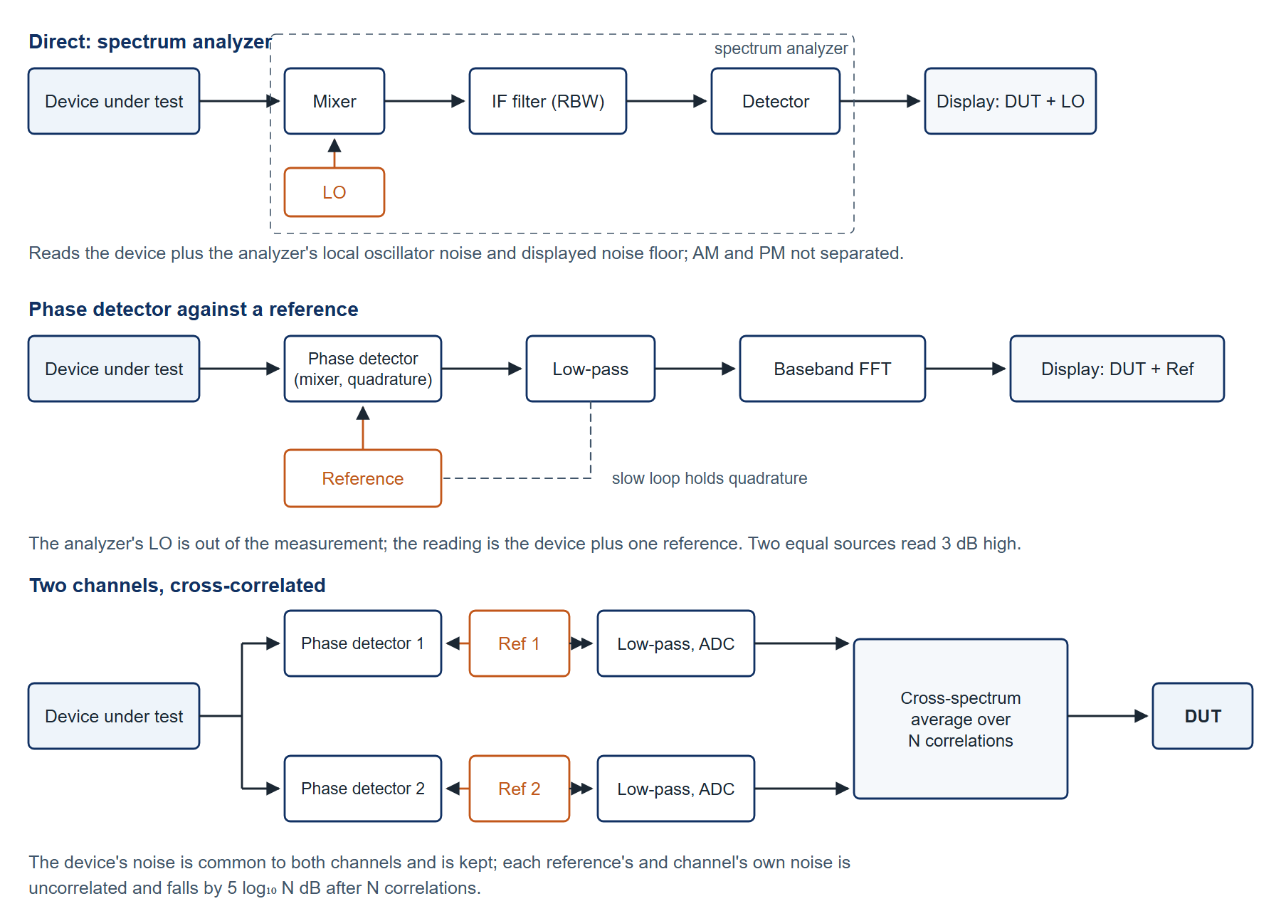
Figure 2. Schematic. The three measurement architectures. Direct measurement sees the device plus the analyzer's own local oscillator; a phase detector sees the device plus one reference; cross-correlation uses two references, and averaging the cross-spectrum removes the noise that is not common to both channels, which is everything except the device. — PhotoFigure 2. **Figure 2.** Schematic. The three measurement architectures. Direct measurement sees the device plus the analyzer's own local oscillator; a phase detector sees the device plus one reference; cross-correlation uses two references, and averaging the cross-spectrum removes the noise that is not common to both channels, which is everything except the device.

Direct measurement on a spectrum analyzer. The analyzer tunes across the carrier and displays the skirts. It is quick, it covers any carrier the analyzer tunes to, and it needs no second source, which is why it is the first measurement made on most benches. What it displays is the device's noise added to the analyzer's own: its local oscillator's phase noise and its displayed noise floor. The displayed value exceeds the device's true value by 10 log₁₀(1 + 10^−m/10), where m is the margin in dB by which the device is noisier than the analyzer. With a 10 dB margin the reading is 0.41 dB high; with 3 dB it is 1.76 dB high; with no margin the reading is 3 dB high and the measurement is of the analyzer. The architecture also cannot separate amplitude noise from phase noise, because a swept detector responds to both, and the reading has to be normalized from the resolution bandwidth to 1 Hz and corrected for the detector's response to noise; the analyzer's noise marker does both. The restriction, then, is that direct measurement is a measurement of the device only where the device is clearly noisier than the analyzer, which excludes exactly the sources a designer most wants to characterize: good oscillators, reference-grade synthesizers and clocks.

A phase detector against a reference. Mixing the device with a reference at the same frequency, held in phase quadrature by a slow phase-locked loop, produces a baseband voltage proportional to the phase difference. A baseband analyzer then measures that voltage's spectrum, and dividing by the detector constant gives S_φ(f). The spectrum analyzer's LO is no longer in the measurement at all, so the floor can be tens of decibels below any direct measurement, and amplitude noise is rejected by the quadrature condition. The limit is the reference: the detector output carries the device's phase noise plus the reference's, and two equal sources read 3 dB high. The method also needs the loop's bandwidth accounted for close to the carrier, where the loop suppresses the very noise being measured.

Two channels, cross-correlated. Build two phase-detector channels, each with its own independent reference, and feed the device to both. The device's phase noise appears identically in both channels; each reference's noise, and each channel's own electronics noise, appears in only one. Averaging the cross-spectrum of the two channels over N measurements keeps the common part and reduces the uncorrelated part by 5 log₁₀ N dB: about 5 dB for 10 correlations, 10 dB for 100, 15 dB for 1000, which is the figure the 7000 Series datasheet gives. The device's noise is not averaged away, because it is common to both channels. The price is time. Each correlation takes a fixed time that depends on the lowest offset measured, and the total is the number of correlations times that figure. Table 2 gives the published times for one correlation.

**Table 2.**
Measurement range	Time per correlation	100 correlations	1000 correlations
0.1 Hz to 100 MHz	80 s	2.2 h	22 h
1 Hz to 100 MHz	8 s	13 min	2.2 h
10 Hz to 100 MHz	0.8 s	80 s	13 min
100 Hz to 100 MHz	0.1 s	10 s	100 s
1 kHz to 100 MHz	0.01 s	1 s	10 s
10 kHz to 100 MHz	below 0.004 s	below 0.4 s	below 4 s

Cross-correlation is therefore a trade of measurement time for floor. A floor 15 dB below a single channel's costs a thousand correlations, which is 13 minutes when the measurement starts at 10 Hz and 22 hours when it starts at 0.1 Hz. The time is spent at the low-offset end, so the practical rule is to start the offset range no lower than the application needs.

4. Reading a sensitivity table before trusting a plot

The criterion for any phase noise measurement, by any of the three architectures, is the same: the instrument's floor at the carrier frequency, at the offsets that matter to the application, after the number of correlations the time budget allows, must be at least 10 dB below the noise the device is expected to show. At 10 dB the reading is 0.41 dB high, which is inside the instrument's own accuracy specification; at less than that the floor is part of the answer and has to be subtracted, which is possible only when it is known precisely.

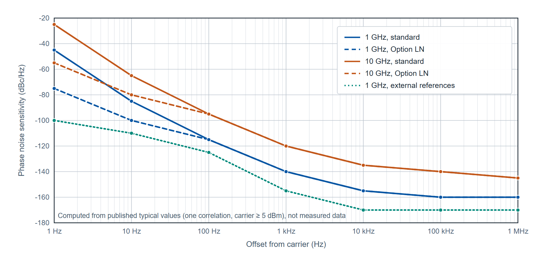
A sensitivity table is how a vendor publishes that floor, and it is read as a grid: carrier frequency down the side, offset across the top, floor at the intersection, with the number of correlations and the carrier power it applies to stated in the heading. The floor rises with carrier frequency, because the internal references are multiplied up to the carrier and their noise rises by 20 log₁₀ of the multiplication ratio, and it falls with offset until it reaches the white floor. Figure 3 draws the published 7000 Series floors at 1 GHz and 10 GHz, with the standard internal references and with Option LN, after one correlation. Table 3 gives the rows the figure is drawn from.

Figure 3. Derived. 7000 Series absolute phase noise sensitivity at 1 GHz and 10 GHz carriers with the standard internal references and with Option LN, after one cross-correlation, carrier power 5 dBm or more. Computed from the published typical values in Table 3, joined log-linearly. Option LN lowers the floor inside 100 Hz; the floors beyond 1 kHz are the same for both. — PhotoFigure 3. **Figure 3.** Derived. 7000 Series absolute phase noise sensitivity at 1 GHz and 10 GHz carriers with the standard internal references and with Option LN, after one cross-correlation, carrier power 5 dBm or more. Computed from the published typical values in Table 3, joined log-linearly. Option LN lowers the floor inside 100 Hz; the floors beyond 1 kHz are the same for both.

**Table 3.**
Carrier, references	1 Hz	10 Hz	100 Hz	1 kHz	10 kHz	100 kHz	1 MHz
1 GHz, standard	−45	−85	−115	−140	−155	−160	−160
1 GHz, Option LN	−75	−100	−115	−140	−155	−160	−160
10 GHz, standard	−25	−65	−95	−120	−135	−140	−145
10 GHz, Option LN	−55	−80	−95	−120	−135	−140	−145
1 GHz, external references	−100	−110	−125	−155	−170	−170	−170

Three things to read from the table. First, the gap between the 1 GHz and 10 GHz rows is 20 dB at every offset, which is 20 log₁₀(10), the multiplication penalty. A device at 6 GHz is measured against a floor between the two rows, and the safe assumption is the worse one. Second, Option LN changes only the two left-hand columns: it is a close-in improvement, and it buys nothing at 1 kHz and beyond. Third, an external reference of higher quality than the internal ones lowers the floor at every offset, which is why the last row is the lowest; the external-reference path is available from 5 MHz to 18 GHz on the 7300 and 7340 and from 5 MHz to 7 GHz on the 7070.

The far-out floor has a second limit that no number of correlations removes: thermal noise. The datasheet states a thermal floor of −177 dBm/Hz, so the floor in dBc/Hz at wide offsets is −177 minus the carrier power in dBm: −177 dBc/Hz for a 0 dBm carrier and −187 dBc/Hz at +10 dBm. The sensitivity tables are stated at a carrier power of 5 dBm or more for this reason, and a device that can only deliver −10 dBm is measured against a floor 15 dB higher than the table at the offsets where thermal noise dominates.

5. Worked example: what the floor adds to an integrated measurement

The question a sensitivity table does not answer directly is how much the floor contributes to an integrated result, which is the figure a clock or link budget uses. Integrating the floor itself over the reporting band gives that contribution as an equivalent rms phase and jitter, and it shows where in the band the contribution comes from.

Take the 1 GHz rows of Table 3 and integrate equation (2) from 10 Hz to 1 MHz, treating the curve as straight in dB against log offset between the tabled points. Each segment integrates in closed form: for a segment from f₀ to f₁ with a slope of m dB per decade and a linear value L₀ at f₀, the integral is L₀ f₀ [(f₁/f₀)^a+1 − 1] / (a + 1) with a = m/10. For the standard references:

10 Hz to 100 Hz, −85 to −115 dBc/Hz (−30 dB per decade): 1.57 × 10⁻⁸
100 Hz to 1 kHz, −115 to −140 (−25 dB per decade): 2.04 × 10⁻¹⁰
1 kHz to 10 kHz, −140 to −155 (−15 dB per decade): 1.37 × 10⁻¹¹
10 kHz to 100 kHz, −155 to −160 (−5 dB per decade): 1.37 × 10⁻¹¹
100 kHz to 1 MHz, flat at −160: 10⁻¹⁶ × 9 × 10⁵ = 9.0 × 10⁻¹¹

The sum is 1.60 × 10⁻⁸; doubling it for both sidebands gives φ_rms² = 3.19 × 10⁻⁸ rad², so φ_rms = 1.79 × 10⁻⁴ rad = 0.0102 degrees, and by equation (3) the equivalent jitter at 1 GHz is 1.79 × 10⁻⁴ / (2π × 10⁹) = 28.4 fs. Figure 4 draws the curve with the integrated band shaded.

Figure 4. Derived. The 1 GHz floors of Table 3 from 10 Hz to 1 MHz with the integrated band shaded. Computed from published typical values, not measured data. With the standard references 98 percent of the integral lies in the 10 Hz to 100 Hz decade, and the floor's equivalent jitter is 28 fs after one correlation; with Option LN the same decade holds 81 percent and the equivalent jitter is 9.3 fs. — PhotoFigure 4. **Figure 4.** Derived. The 1 GHz floors of Table 3 from 10 Hz to 1 MHz with the integrated band shaded. Computed from published typical values, not measured data. With the standard references 98 percent of the integral lies in the 10 Hz to 100 Hz decade, and the floor's equivalent jitter is 28 fs after one correlation; with Option LN the same decade holds 81 percent and the equivalent jitter is 9.3 fs.

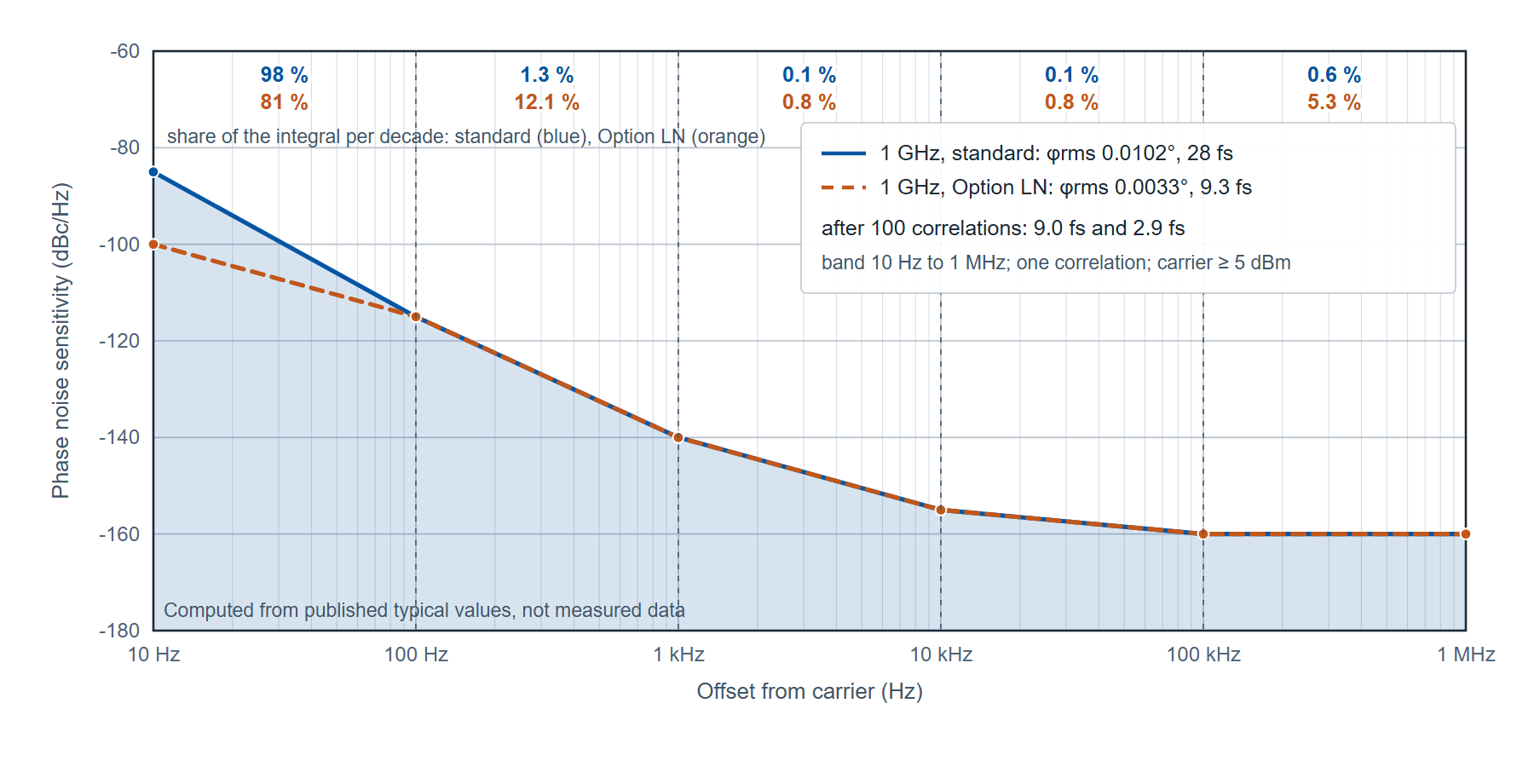
The first segment holds 98 percent of the total. That is the general property of a curve that falls at 30 dB per decade: the integral is dominated by its lowest decade, so the floor's contribution to an integrated figure is set almost entirely by the close-in columns of the table, and the reporting band's lower limit decides the answer. The same arithmetic for the Option LN row, which differs only at 10 Hz (−100 instead of −85), gives φ_rms = 5.81 × 10⁻⁵ rad, or 9.3 fs: a 15 dB change in one column reduced the integrated floor by a factor of three.

Correlations act on the whole curve at once. After 100 correlations the floor is 10 dB lower at every offset, so every segment integral falls by a factor of 10 and φ_rms by √10: 9.0 fs with the standard references and 2.9 fs with Option LN. In measurement time, from Table 2, 100 correlations starting at 10 Hz cost 80 s. A clock specified at 50 fs over 10 Hz to 1 MHz can therefore be measured on the standard references after one correlation with the floor contributing 28 fs, which when subtracted in quadrature changes a 50 fs reading by 9 fs, or after 100 correlations with the floor contributing 9 fs, which changes it by 0.8 fs. The second measurement costs 79 s more and removes the subtraction.

This is also what the two sensitivity plots in the 7000 Series datasheet show, labeled "after 1 correlation" and "after 100 correlations": the second is the first lowered by about 10 dB at every point, and the per-decade shares above say why that matters more close in than far out.

6. The 7000 Series as an instance of the architecture

The 7000 Series Signal Source Analyzer is a two-channel cross-correlation instrument with two internal tunable references, and it accepts external references as well. Three models share the chassis, software and option set and differ in top frequency: the 7070 measures from 1 MHz to 7 GHz, the 7300 from 1 MHz to 26 GHz and the 7340 from 1 MHz to 40 GHz, the last with a K (2.92 mm) input connector and the others with SMA. Offsets run from 0.01 Hz to 100 MHz. Measurement accuracy is ±4 dB below 10 Hz offset, ±3 dB from 10 Hz to 1 kHz and ±2 dB from 1 kHz to 100 MHz. The input accepts −15 to +20 dBm below 18 GHz and −15 to +23 dBm from 18 to 30 GHz, with a damage level of +26 dBm. Internal spurious is −90 dBc with the internal references. Figure 5 shows the instrument.

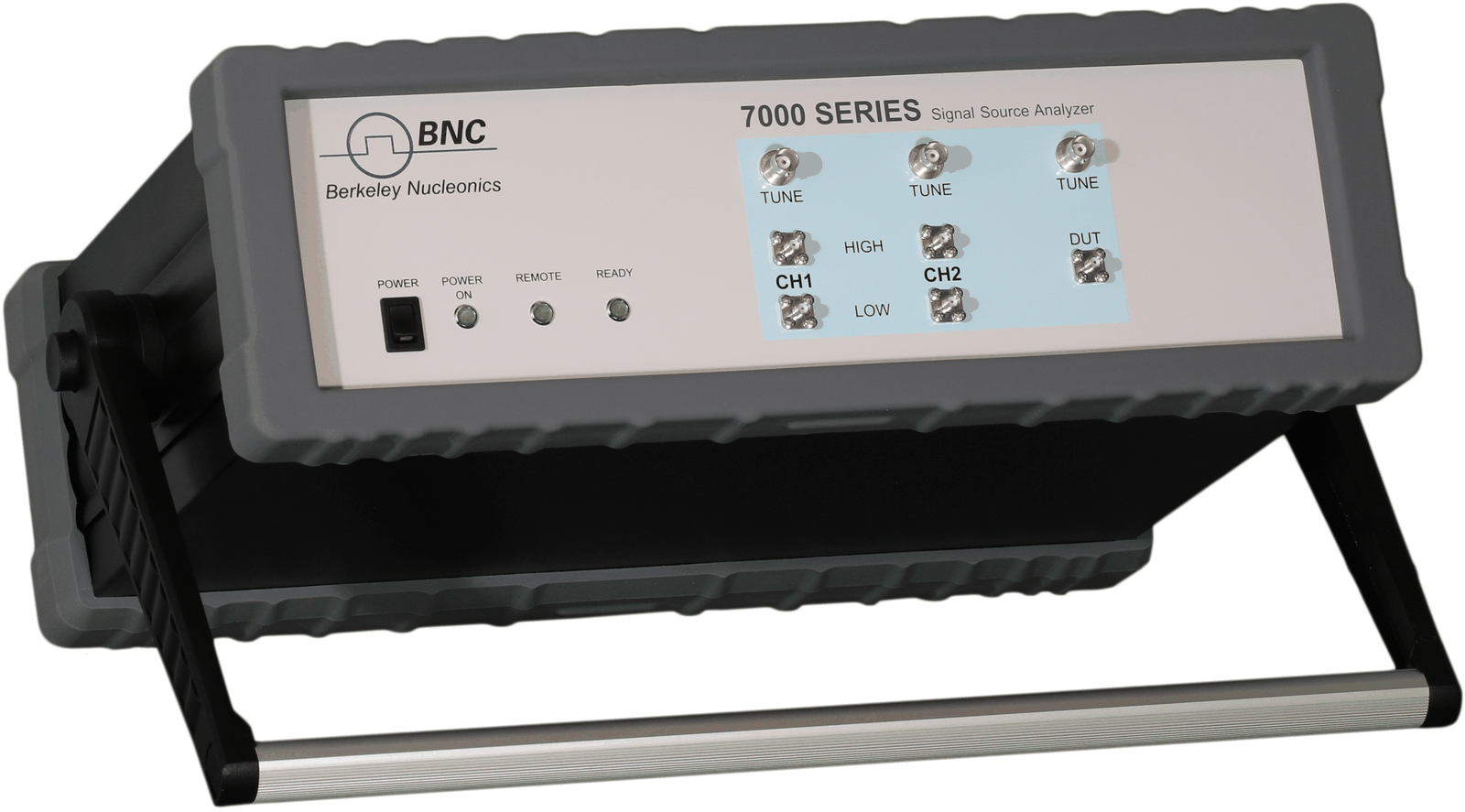
Figure 5. Photo. The 7000 Series Signal Source Analyzer: a 3U half-rack instrument with the two reference channels and the device-under-test connections on the front panel. — PhotoFigure 5. **Figure 5.** Photo. The 7000 Series Signal Source Analyzer: a 3U half-rack instrument with the two reference channels and the device-under-test connections on the front panel.

Absolute phase noise is the standard mode, reporting L(f), spurs, integrated rms phase in degrees and radians, time jitter and residual FM. The same hardware measures residual (additive) phase noise of two-port devices such as amplifiers and dividers (Option APN), pulsed and burst phase noise (Options PULSE, NPS and BURST), amplitude noise (Option AM), baseband noise on two rear inputs from 1 Hz to 100 MHz, transient frequency and phase against time (Option TRAN), Allan deviation (Option TSTAB) and spectrum monitoring (Option SPEC). Two programmable low-noise DC supplies (0 to 15 V, 550 mA per channel) and three tuning voltages (−5 to +20 V) power and tune a device under test from the instrument, which removes the bench supply from the measurement; Option VCO sweeps the tuning voltage and logs frequency, tuning sensitivity, pushing, output power, supply current and phase noise at each point. Control is by LAN (VXI-11), USBTMC or optional GPIB with a SCPI command set, an API library and the platform-independent GUI.

Which model and options a given job needs follows from section 4. The top frequency is the carrier range; Option LN is for close-in work on good sources, where the two left-hand columns of Table 3 matter; the external-reference path is for the lowest floors on carriers up to 18 GHz; and the time per correlation in Table 2 sets how many correlations a production test can afford.

7. Measurement practice

These steps apply to any phase noise measurement and to any instrument.

Warm up to the specification condition. The 7000 Series specifications hold at 23 ±5 °C after a 30 minute warm-up; the device under test usually needs as long, and an oven-controlled oscillator needs longer.
Set the input level inside the published range and as high as the device delivers cleanly, because the far-out floor is thermal noise relative to the carrier. Check the damage level before connecting a power amplifier output.
Use short, torqued, phase-stable cables at the carrier, and keep the device, its supply and the analyzer on one ground. A supply ripple line or a ground loop appears as a spur, and a spur is reported separately from the noise.
Choose the offset range from the application, not from the instrument: start it at the lowest offset the application integrates from, since the time per correlation is set by that start (Table 2).
Choose the number of correlations from the floor margin: enough that the instrument floor is 10 dB below the expected device noise at every offset of interest. Check the margin against the sensitivity table, at the carrier frequency, before the measurement rather than after.
Read spurs from the spur table in dBc, not from the trace in dBc/Hz, and record which were excluded from the integration.
Report the integrated phase with its band, the number of correlations, the carrier power and the reference used. A plot without these cannot be compared with another.

8. Limitations

Cross-correlation lowers the instrument's uncorrelated noise; it does not lower the device's, and it does not remove a reference spur that is coherent in both channels. Its cost grows with the lowest offset: a 0.1 Hz measurement takes 80 s per correlation, so a thousand-correlation result at that offset is a day's measurement. Close to the carrier the published accuracy is ±4 dB below 10 Hz and ±3 dB to 1 kHz, which bounds what any close-in comparison between two devices can resolve. The external-reference path, which gives the lowest floors, covers 5 MHz to 18 GHz on the 7300 and 7340; above 18 GHz the internal references set the floor. And the thermal floor at wide offsets is set by the device's own output power, not by the instrument.

There is also a case where the instrument is not needed. A source whose phase noise is 20 dB or more above a good spectrum analyzer's LO noise and displayed noise at the offsets of interest, such as a free-running VCO or a wideband fractional-N synthesizer far from its loop bandwidth, reads within 0.04 dB on the direct method. For that device a spectrum analyzer with a noise marker is a correct instrument, and a cross-correlation analyzer earns its place only when the device improves to within 10 dB of the analyzer's floor.

Summary

L(f) = ½ S_φ(f), in dBc/Hz, is the noise power in a 1 Hz band at offset f, relative to the carrier; spurs are discrete and reported in dBc.
Integrated rms phase is 2 ∫ L(f) df over a stated band; jitter is φ_rms / (2π f₀). On a curve falling at 30 dB per decade the lowest decade dominates the integral.
A floor 10 dB below the device adds 0.41 dB to the reading; an equal floor adds 3 dB.
Cross-correlation lowers the uncorrelated instrument noise by about 5 dB per decade of correlations (10 dB at 100) at a cost of correlations times the time per correlation (0.8 s from 10 Hz; 8 s from 1 Hz; 80 s from 0.1 Hz).
7000 Series published floor at 1 GHz, standard references, one correlation: −85 dBc/Hz at 10 Hz, −140 at 1 kHz, −160 at 100 kHz; equivalent jitter 10 Hz to 1 MHz 28 fs (9.3 fs with Option LN; 9.0 and 2.9 fs after 100 correlations).
Thermal floor −177 dBm/Hz, so the far-out floor in dBc/Hz is −177 minus the carrier power in dBm.
7070: 1 MHz to 7 GHz; 7300: 1 MHz to 26 GHz; 7340: 1 MHz to 40 GHz. Offsets 0.01 Hz to 100 MHz. Accuracy ±4, ±3 and ±2 dB below 10 Hz, to 1 kHz and above 1 kHz.

Definitions

Additive (residual) phase noise. The phase noise a two-port device such as an amplifier adds to a signal passing through it, measured with the source noise cancelled.

Correlation. One averaged measurement of the cross-spectrum of the two channels of a cross-correlation analyzer; the uncorrelated noise falls by 5 log₁₀ N dB after N of them.

dBc/Hz. Decibels relative to the carrier power, in a 1 Hz bandwidth; the unit of L(f).

Integrated phase noise. The rms phase error obtained by integrating L(f) over a stated band; meaningless without the band.

Offset frequency. The distance from the carrier at which L(f) is evaluated, in Hz.

Reciprocal mixing. The transfer of a local oscillator's phase noise onto a strong adjacent signal, which then falls into the wanted channel.

Single-sideband phase noise, L(f). Half the one-sided spectral density of phase fluctuation, per IEEE Std 1139.

Spur. A discrete spectral line at a fixed offset, with a fixed power; reported in dBc.

Time jitter. The rms phase error expressed in time at the carrier frequency.

Symbols

**Table 4.**
Symbol	Meaning	Unit
L(f)	Single-sideband phase noise at offset f	dBc/Hz, or a linear ratio per Hz in the integral
S_φ(f)	One-sided spectral density of phase fluctuation	rad²/Hz
f	Offset from the carrier	Hz
f₀	Carrier frequency	Hz
f_L, f_H	Lower and upper limits of the integration band	Hz
φ_rms	Integrated rms phase error	rad (or degrees)
t_j	rms time jitter	s
m	Margin of the device noise above the instrument floor	dB
N	Number of correlations	none

Acronyms

AM amplitude modulation or amplitude noise. API application programming interface. DUT device under test. FFT fast Fourier transform. GUI graphical user interface. LN low noise (Option LN, the ultra-low-noise internal references). LO local oscillator. PLL phase-locked loop. QAM quadrature amplitude modulation. RBW resolution bandwidth. SCPI Standard Commands for Programmable Instruments. SSB single sideband. VCO voltage-controlled oscillator.

Discuss your phase noise measurement

Berkeley Nucleonics builds the 7000 Series phase noise analyzers and signal source analyzers and offers them for sale and rent. Our application engineers would be glad to talk through a measurement, from the floor margin at your carrier to the number of correlations a production test can afford: request a quote or demo, write to info@berkeleynucleonics.com, or call 800-234-7858.

Phase noise measurement basics: what the number means and how it is measured