What "power" means for a real signal
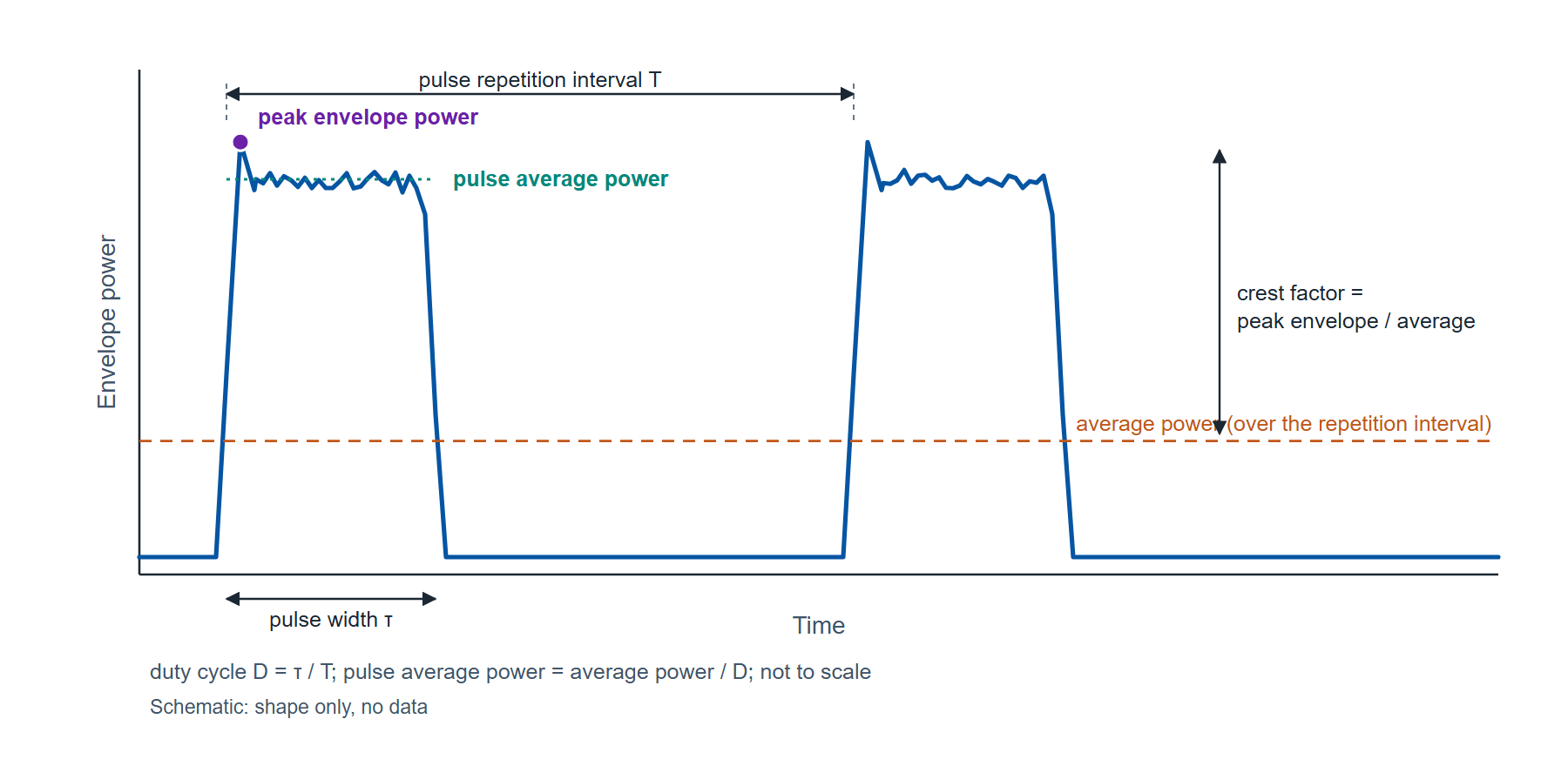
A continuous-wave carrier has one power. A modulated or pulsed signal has several, and a sensor reading is only as useful as the agreement about which one it reports. The instantaneous power rises and falls at twice the carrier frequency. The envelope power is its average over a few carrier cycles, the quantity that follows the modulation. The average power is the envelope power averaged over the modulation, or over many pulses. For a pulsed carrier two more are needed: the pulse average power, the average over the pulse alone, and the peak envelope power, the highest value the envelope reaches. Figure 1 draws all of them on one pulsed waveform.
The relations between them are arithmetic, and for a periodic pulse train with a flat top they are exact:
where D is the duty cycle (0.01 for a 10 µs pulse every 1 ms), τ is the pulse width, T is the pulse repetition interval, Pavg is the average power over T, Ppulse is the pulse average power, Ppeak is the peak envelope power, and CF is the crest factor, also called the peak-to-average power ratio (PAPR). All powers are linear (watts) in these relations; in decibels the division becomes a subtraction.
A worked case: a radar-type train of 10 µs pulses at a 1 ms interval has D = 10 µs / 1 ms = 0.01. A true-RMS average sensor reads Pavg = −10.0 dBm, which is 0.100 mW. The pulse average power is 0.100 mW / 0.01 = 10.0 mW, or +10.0 dBm, which is the average reading plus 10 log10(1/D) = +20 dB. The result is exact only when the pulse top is flat and the duty cycle is known: a 10 percent error in D is a 10 log10(1.1) = 0.41 dB error in Ppulse, so the duty cycle should come from a counter or the generator setting, not from an estimate.
How a diode sensor detects power
The RF signal is terminated in a 50 Ω load, and a high-frequency diode pair rectifies the voltage across it. At low input levels the diode operates in its square-law region, where the DC output is proportional to the square of the RF voltage and therefore to power. In that region the detector responds to the mean-square voltage of whatever waveform is applied, so its reading is the true RMS average power regardless of modulation: a CW carrier, an OFDM signal with a high crest factor and a pulse train with the same average power all produce the same DC output. At higher levels the diode leaves square law and the output follows the envelope voltage instead, where the reading depends on the waveform's shape. An average power sensor keeps the detector in square law across its whole range, by sensing and conditioning the input, and the sensor's processing applies a linearization and a calibration factor against frequency before the result leaves it over USB. Figure 2 draws the chain.
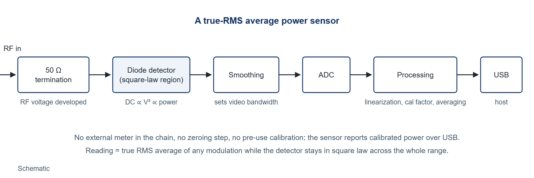
The smoothing after the detector sets the sensor's video bandwidth, the rate at which its output can follow the envelope. For a single-pole response the rise time and the bandwidth are tied by tr ≈ 0.35 / Bv, an approximation that holds for a first-order low-pass response and is used here as such. A video bandwidth of 10 kHz corresponds to a rise time of 0.35 / 10 kHz = 35 µs; 60 kHz corresponds to 5.8 µs. Envelope features faster than the rise time are averaged by the sensor, which is what an average sensor is for and what makes it the wrong instrument for a pulse's edges.
What an average sensor measures, and what it does not
An average sensor measures the average power of any modulation, with an accuracy that does not depend on the crest factor. Operated with a trigger and a gate, it also measures the average over a defined window, which recovers the pulse average power directly when the gate spans a whole pulse and the video bandwidth is wide relative to the pulse. It does not measure peak envelope power, rise time, overshoot or droop. Those are the properties of a pulse's shape, and they need a peak power sensor whose video bandwidth is several times wider than the fastest edge; for a 100 ns rise time that is a video bandwidth above 3.5 MHz, two orders beyond an average sensor's. The division is clean: average and pulse-average power with the sensor described here, pulse profile with a peak sensor.
Before the product, the criterion. An average sensor is specified by its frequency range and connector; its dynamic range; its linearity and calibration-factor uncertainty, which together with mismatch make up the measurement uncertainty; its zero offset and its noise, which set the floor and how averaging lowers it; its three input limits, continuous average, peak and energy per pulse, all of which must be respected at once; and its measurement rate, which sets how many readings a test can take in a second. A sensor that is read against those seven items can be compared with any other.
The Model 12100 Series as the instance
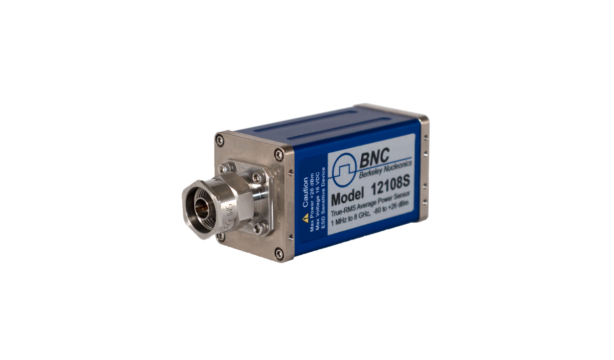
The Model 12100 Series is a family of USB-powered true-RMS average power sensors. Each model sets its frequency reach and connector: 9 kHz (L build) or 1 MHz (S build) to 8 GHz with Type-N, to 18 GHz with Type-N, to 26.5 GHz with 3.5 mm, to 40 GHz with 2.92 mm, to 44, 50 and 54 GHz with 2.4 mm and to 67 GHz with 1.85 mm, and the Model 12175 covers 50 to 75 GHz in WR-15 waveguide. The dynamic range is −60 to +26 dBm across the coaxial family, which is 1 nW to about 400 mW, a span of 86 dB; the 12175 covers −50 to +18 dBm. The sensor needs no external meter, no zeroing and no pre-use calibration, and the specifications hold after a 30 minute warm-up for CW signals unless stated otherwise. Table 1 collects the published figures the criterion above asks for.
| Item | Published value | Condition |
|---|---|---|
| Input power range | −60 to +26 dBm | Coaxial models; 12175: −50 to +18 dBm |
| Continuous average limit | +26 dBm (400 mW); damage +29 dBm (800 mW) | 12167L and 12175: +18 dBm, damage +23 dBm |
| Peak power limit | +23 dBm (200 mW); damage 36 dBm (4 W) | 12167L: +26 dBm; 12175: +18 dBm, damage +23 dBm |
| Energy per pulse limit | 20 W·µs; damage 40 W·µs | 12167L: 5 W·µs, damage 10 W·µs |
| Linearity uncertainty | 2.0 % (−10 to +10 dBm); 3.0 % (+10 to +20 dBm); 3.5 % (−20 to −10 dBm); 2.0 % (−60 to −20 dBm) | Average mode; Normal detector mode adds 1 to 1.5 % to the calibration-factor figures on S builds |
| Noise, Average mode | 0.35 % of reading (−40 to +26 dBm); 0.5 nW (−60 to −40 dBm), typical 0.2 nW | Two standard deviations of 100 points; scales as 4 / √(averages) |
| Zero offset, Average mode | 1.0 nW at 25 °C, plus 0.075 nW per °C away from 25 °C, ±0.01 nW per month | All models |
| Temperature uncertainty | 0 % (20 to 30 °C); 0.5 % (10 to 20 and 30 to 40 °C); 2.5 % (0 to 10 and 40 to 55 °C) | Average mode |
| Measurement rate, Average mode | Normal 38.4 ms per average (384 samples); Double 19.2 ms; Fast 3.2 ms; Super 1.6 ms (16 samples) | Averages 1 to 1024 (Super: to 4069) |
| Video bandwidth, Normal detector mode | 8 kHz minimum, 10 kHz typical; 40 kHz minimum, 60 kHz typical in the top range | Top range about −15 dBm to +26 dBm |
| Interfaces | USBTMC, USB HID; optional SPI or I2C; SCPI command set | PowerEye software supplied |
Four of those rows turn into working limits once a signal is put against them.
The three input limits apply together. A 1 W, 10 µs pulse carries 1 W × 10 µs = 10 W·µs, inside the 20 W·µs energy limit, and 1 W is +30 dBm, which exceeds the +23 dBm peak limit, so that pulse cannot be applied directly even though its energy is allowed; an attenuator of at least 7 dB brings the peak to +23 dBm and the energy to 2 W·µs. An OFDM-class signal with a 10 dB crest factor at an average of +13 dBm reaches peaks of +23 dBm, the limit, so +13 dBm is the highest average at which such a signal can be measured without attenuation, even though the average range runs to +26 dBm.
Zero offset sets the usable bottom of the range. Zero-offset uncertainty as a share of the reading is Z = (zero offset power / measured power) × 100 percent. At 25 °C the offset is 1.0 nW: at −60 dBm (1 nW) it is 100 percent of the reading, at −50 dBm (10 nW) 10 percent, at −40 dBm (100 nW) 1 percent, and at −30 dBm 0.1 percent. At 35 °C the offset is 1.0 + 10 × 0.075 = 1.75 nW and those shares become 175, 17.5, 1.75 and 0.175 percent. The bottom 10 to 20 dB of the range is therefore where zero offset dominates the uncertainty, and a measurement that needs 1 percent should be made above −40 dBm at room temperature.
Averaging buys noise floor at the cost of time. Below −40 dBm the noise specification is 0.5 nW at the Normal rate's 16 averages, and it scales as 0.5 nW × 4 / √N: 0.177 nW at 128 averages and 0.062 nW at 1024, with the typical 0.2 nW figure scaling to 0.071 and 0.025 nW. At 1024 averages in Normal mode each result takes 1024 × 38.4 ms = 39 s. Above −40 dBm the noise is 0.35 percent of the reading, 0.35 nW at −40 dBm, and averaging is rarely needed.
Video bandwidth bounds what a gated measurement can resolve. With a typical 10 kHz video bandwidth the rise time is 35 µs; in the top range at 60 kHz it is 5.8 µs. A gated average over a 10 µs pulse in the top range is therefore valid only if the gate is placed after the response has settled, and at 10 kHz a 10 µs pulse is not resolved at all, which is when the duty-cycle method of equation (1) is used instead.
Measurement practice
- Warm up for 30 minutes; the sensor stabilizes for general use in 5 minutes, but the specifications hold only after 30.
- Set the measurement frequency in the software so the correct calibration factor is applied; the factor's uncertainty is published per band and model.
- Check the signal against all three limits, continuous average, peak and energy per pulse, using its crest factor or its pulse width and amplitude, and add attenuation where any one is exceeded.
- Choose the measurement rate and the number of averages from the noise target: Super or Fast for throughput above −40 dBm, Normal with 128 to 1024 averages for the lowest 20 dB.
- Keep the reading above −40 dBm where 1 percent accuracy is needed, or account for the zero offset at the operating temperature from the formula.
- Record frequency, rate, averages, temperature and the attenuation in the path with every logged value, so a later reading can be compared with it.
Limitations
An average sensor reports no pulse profile: peak envelope power, rise and fall times, overshoot and droop are outside its reach, and a job whose output is those numbers needs a peak power sensor regardless of what else is on the bench. Its gated measurements are bounded by the video bandwidth, 35 µs rise time at the typical 10 kHz. The lowest 10 to 20 dB of the dynamic range is governed by zero offset and noise rather than by linearity, and that floor moves with temperature at 0.075 nW per degree. The published uncertainties are for CW after warm-up; a modulated signal adds the duty-cycle or crest-factor arithmetic above, and that arithmetic is only as good as the duty cycle or crest factor that goes into it.
Summary
- Pulse average power = average power / duty cycle; a 10 µs pulse every 1 ms reading −10.0 dBm average is +10.0 dBm pulse average; a 10 percent duty-cycle error is 0.41 dB.
- Crest factor = peak envelope power / average power; a 10 dB crest factor reaches the +23 dBm peak limit at +13 dBm average.
- Rise time ≈ 0.35 / video bandwidth (single-pole approximation): 35 µs at 10 kHz, 5.8 µs at 60 kHz.
- Zero offset 1.0 nW at 25 °C plus 0.075 nW per °C: 10 percent of a −50 dBm reading, 1 percent at −40 dBm.
- Noise below −40 dBm: 0.5 nW scaling as 4 / √N, 0.062 nW at 1024 averages (39 s in Normal mode).
- Model 12100 Series: 9 kHz or 1 MHz to 8 through 67 GHz by model, 12175 to 75 GHz; −60 to +26 dBm; limits +26 dBm average, +23 dBm peak, 20 W·µs per pulse (model exceptions in Table 1).
Definitions
Average power. Envelope power averaged over the modulation or over many pulse repetition intervals; what a true-RMS sensor reports.
Crest factor (peak-to-average power ratio). Peak envelope power divided by average power, usually stated in dB.
Duty cycle. Pulse width divided by pulse repetition interval.
Envelope power. Power averaged over a few carrier cycles, so that it follows the modulation but not the carrier.
Peak envelope power. The highest value the envelope power reaches.
Pulse average power. Average power over the pulse alone; average power divided by duty cycle for a flat-topped periodic pulse.
Square-law region. The diode operating region in which DC output is proportional to the square of RF voltage, so the detector responds to power independent of waveform.
Video bandwidth. The bandwidth of the sensor's post-detection response, which sets how fast an envelope change it can follow.
Zero offset. The reading with no RF applied, specified as a power and subtracted from every measurement's uncertainty budget.
Further reading
- Model 12100 Series RF power sensor datasheet (web edition) and the datasheet PDF, v2.5: the source of every figure in Table 1.
- Model 12100 Series user manual: triggered and gated measurement setup in PowerEye.
- Model 12100 power sensor temperature sensitivity and Power sensors for radar and satellite: companion briefs.
- RF Power Measurements, the Berkeley Nucleonics reference book, for the detector physics in more depth.
Discuss your power measurement
Our application engineers would be glad to talk through a measurement, from which model and connector fit the band to how many averages a logging job needs. Write to info@berkeleynucleonics.com, call 800-234-7858, or request a quote or demo.