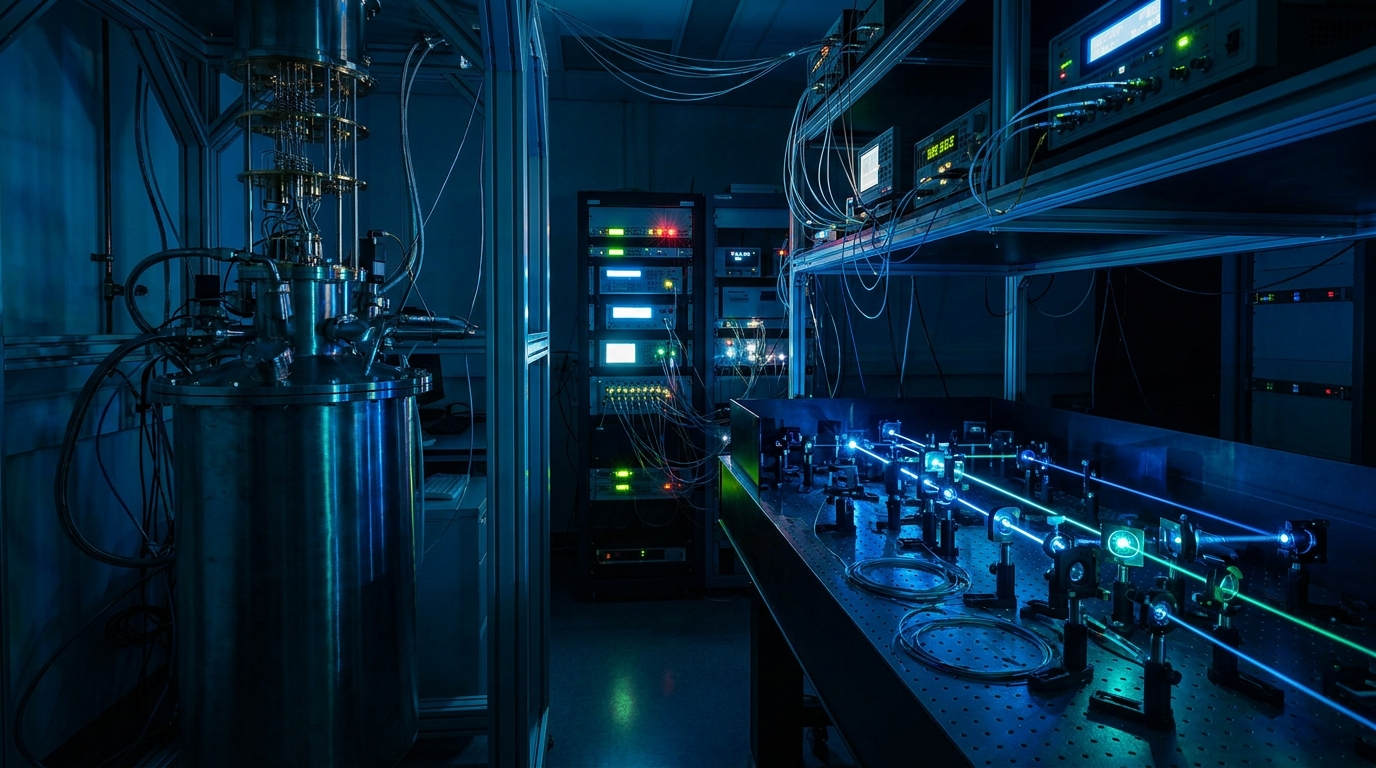
Quantum: QKD & Sensing

That places specific demands on the instrument. The pulses have to land where the protocol expects them, so timing jitter has to be low and the timing grid fine enough to place an edge with confidence. A few picoseconds of uncertainty on a pulse edge can blur the boundary between two encoded states or smear the interrogation window a sensor depends on, and slow drift between channels adds to it over a long run. The sequences themselves are long and often randomized, so a QKD test run or an extended sensing interrogation needs deep waveform memory rather than a short repeating pattern. For protocol development and testing, the record should be long enough that the randomized pattern does not repeat within a measurement, because a repeating pattern correlates with any periodic systematic error in the setup.

Many setups also span more than one channel and more than one modulator. A QKD transmitter may drive an intensity modulator and a phase modulator together, and a multi-qubit experiment drives several control lines at once, so the channels have to stay tightly synchronized against a shared reference rather than drifting apart over the experiment. And the amplitude has to be clean and faithful, because a distorted envelope shows up directly as a degraded quantum state or a noisier measurement. These requirements apply together: low jitter, a fine timing grid, deep memory, multi-channel synchronization and clean amplitude, on the same channels.

How the Model 686 solves it

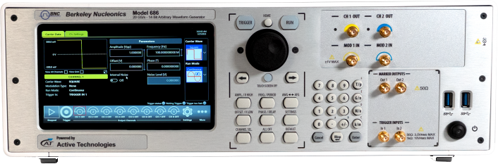
The Model 686 (Figure 2) specifies its timing with conditions that map onto these requirements. Trigger In to output jitter is 0.29 × DAC clock period rms in True Arb mode, 14.5 ps rms at 20 GS/s, and under 20 ps rms in AFG mode; that is the figure to budget when each sequence starts on an external event. Random jitter on a clock pattern is under 2 ps rms; it describes the output edges, not the timing of the output relative to a trigger. To keep the trigger path out of the timing budget, run the 686 from the experiment's reference clock (5 MHz to 500 MHz input) and start the experiment from a 686 marker output, whose jitter is under 10 ps rms. Within one chassis, channel-to-channel skew is adjustable with 100 fs resolution (between CH1 and CH2 on the 2-channel models; between the CH1/CH2 and CH3/CH4 pairs on the 4-channel models), with ±(1% of setting + 20 ps) accuracy and under 20 ps initial skew.

The sample period at 20 GS/s is 50 ps, the grid on which pulse edges and inter-pulse spacing are placed for the encoding and interrogation patterns these protocols use. In True Arb mode at full rate, CH1 holds up to 9.6 Gsamples (CH1 and CH3 on the 4-channel models), 0.48 s of waveform at 20 GS/s; at a 1 GHz pulse rate, with one pulse slot every 20 samples, that is 480 million slots before the record repeats. CH2 holds 1.17 Msamples on the 2-channel models, and CH2 and CH4 hold 589 ksamples on the 4-channel models, so the long randomized sequence belongs on CH1 or CH3. Vertical resolution is 14 bits. The single-ended models deliver up to 5 Vpp into 50 Ω. Where a modulator's required swing is within that, the generator drives it directly, without an external amplifier adding its own noise and delay.

For experiments that outgrow one chassis, up to four units synchronize over the dedicated sync bus (QSFP Sync In and Sync Out, RIDER-686-SYNC cable); four 4-channel units give 16 analog and 128 digital channels. Alignment between units is set during calibration rather than specified: measure the offset between units once at setup and remove it with the channel skew adjustment.

Where amplitude resolution matters more than sample rate, the Model 685 offers 16-bit vertical resolution at up to 6.16 GS/s, with 2 Gsamples of waveform memory per channel (4 Gsamples optional). Its two extra bits give four times as many amplitude levels as the 686, which suits sensing and control work that needs a finely graded envelope more than the fastest edges. The 685 and 686 use different synchronization buses (Infiniband 4X on the 685, QSFP on the 686), so a mixed setup shares one timebase through a common external reference clock, for example 10 MHz, inside both reference input ranges (5 MHz to 200 MHz on the 685, 5 MHz to 500 MHz on the 686).

Choose the Model 685 instead of, or alongside, the 686 when 16-bit vertical resolution matters more than the highest sample rate. Lock every unit, 685 and 686 alike, to the same external reference clock so the full system shares one frequency reference.

For a quick question, chat with an engineer at berkeleynucleonics.com.

Ask now → Chat with our assistant and get an answer in seconds.