Abstract. A data converter records its input at the instant a clock edge arrives, so timing error on the clock becomes voltage error in the data. This note derives the signal-to-noise ratio that clock jitter alone permits, shows how to turn a published phase noise table into an rms jitter figure over a stated band, and lists the six rows of a clock source datasheet that decide whether the source fits a converter. It then works the arithmetic on the published typical values of a low-noise microwave Signal Generator at 1 GHz, with the band limits and the assumptions shown, and closes with a measurement practice section and the limits of the method.
Who this note is for. Design and test engineers characterizing analog-to-digital and digital-to-analog converters, and engineers specifying the clock for a sampled receiver or an arbitrary waveform generator. Test technicians will find the setup and the checklist in the measurement practice section.
11. How timing error becomes voltage error
A converter samples the input voltage at the moment its clock edge crosses threshold. If the edge is early or late by a time Δt, the converter records the voltage the input had at the wrong moment. The error is the input slope at that moment multiplied by the timing error, as Figure 1 shows. The same Δt produces almost no error at the peak of a sine, where the slope is zero, and the largest error at the zero crossing, where the slope is 2πfinA for an input of amplitude A at frequency fin.
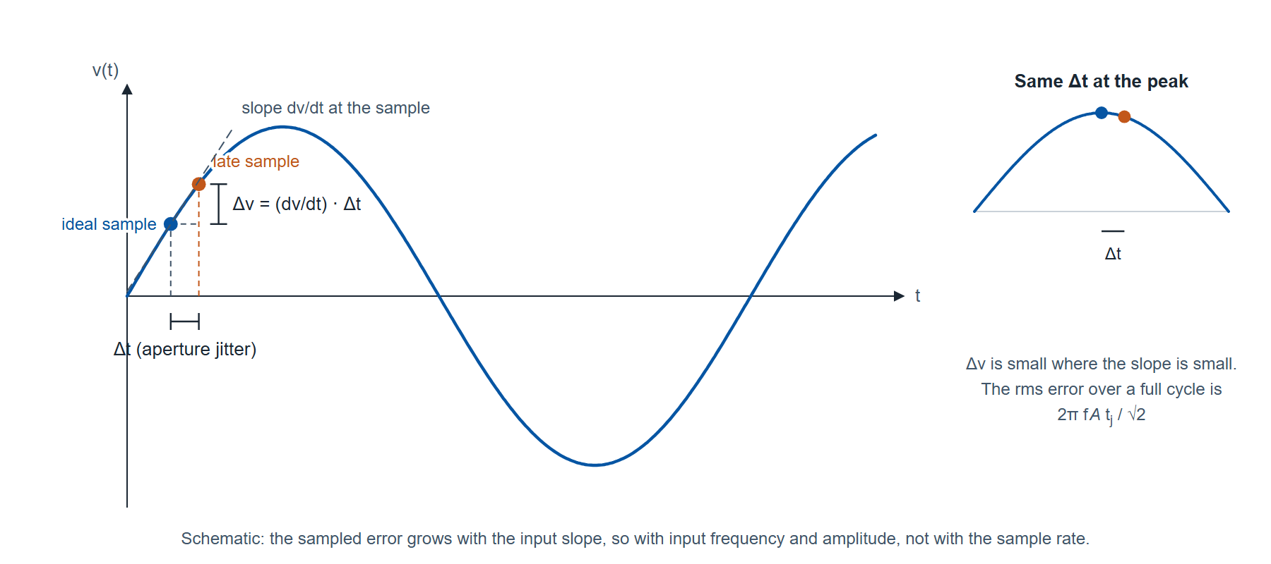
Averaging the slope over a full cycle gives an rms voltage error of 2πfinA tj/√2 for an rms timing error tj, while the signal itself has an rms value of A/√2. The ratio of the two is the signal-to-noise ratio the clock alone allows, with the converter otherwise perfect:
where fin is the input frequency in hertz (1 GHz in the examples below) and tj is the rms clock jitter in seconds, integrated over the band that matters to the converter (section 2).
Equation (1) sets the scale for everything that follows. An ideal N-bit converter has a signal-to-noise ratio of 6.02N + 1.76 dB, which is 74.0 dB for 12 bits and 86.0 dB for 14 bits. Inverting equation (1) for the jitter that holds a 1 GHz input to the 12-bit figure gives tj = 1 / (2π × 109 × 1074/20) = 1 / (6.283 × 109 × 5012) = 31.8 fs. The 14-bit figure needs 1 / (6.283 × 109 × 19,950) = 8.0 fs. At a 100 MHz input the same converters need 318 fs and 80 fs. Figure 2 plots equation (1) across the range a microwave clock serves.
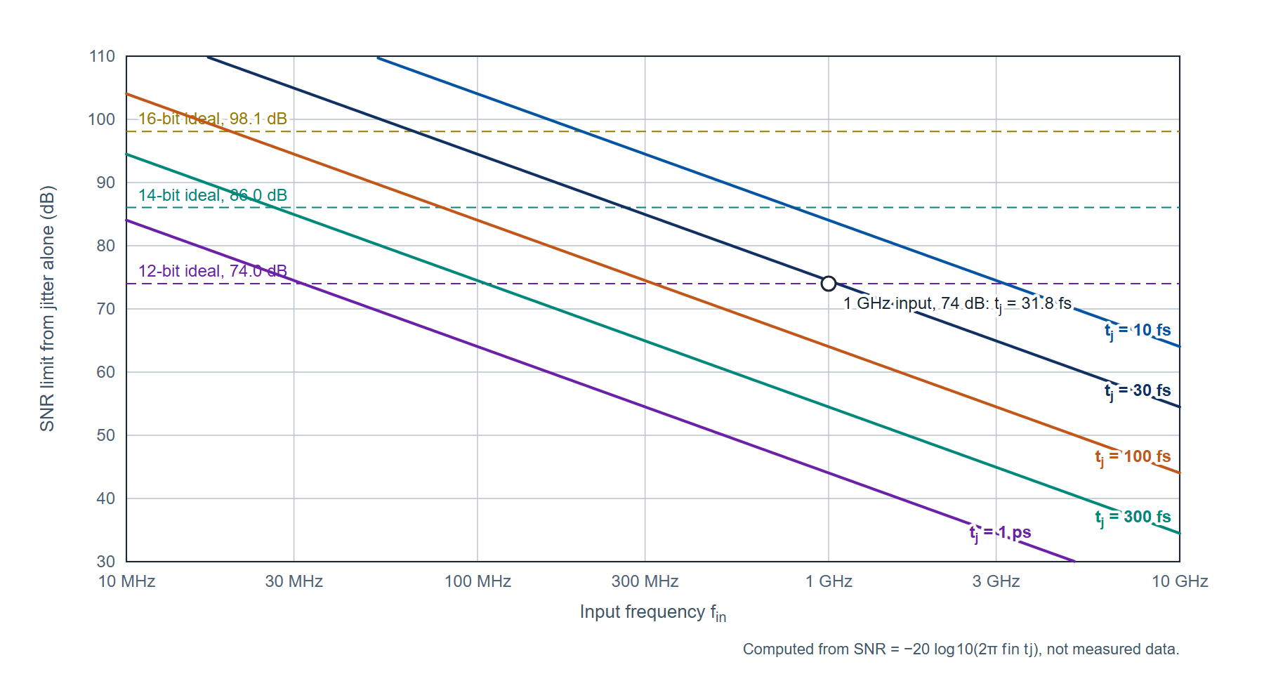
Two consequences follow from the slope argument. The requirement is set by the highest input frequency and not by the sample rate: a receiver that undersamples a 1 GHz intermediate frequency with a 250 MHz clock needs the same 31.8 fs as a converter running at 2.5 GS/s with a 1 GHz input. And the clock jitter adds in power to the converter's own aperture jitter and to its quantization noise, so a clock budget set a few femtoseconds below the line in Figure 2 leaves room for the converter.
22. From a phase noise table to a jitter number
A Signal Generator datasheet states single-sideband phase noise L(f), in dBc/Hz, at a set of offsets f from the carrier. Jitter is the same quantity seen in the time domain. Integrating L(f) over an offset band gives the mean-square phase deviation, and dividing the rms phase by the carrier's angular frequency gives the rms time deviation:
where L(f) is the single-sideband phase noise as a power ratio (10LdB/10, so −130 dBc/Hz is 10−13 per hertz), f1 and f2 are the lower and upper offset limits in hertz, the factor 2 counts both sidebands, φrms is in radians and f0 is the carrier frequency in hertz (the clock frequency, 1 GHz below). The definitions follow IEEE Std 1139.
Between the tabled points the curve is joined on log-frequency, linear-dB segments, and each segment integrates in closed form: on a segment that falls m dB per decade, L(f) = L(fa)·(f/fa)m/10, whose integral from fa to fb is L(fa)·fa·[(fb/fa)m/10+1 − 1] / (m/10 + 1). Section 4 works it on a real table.
The band limits are part of the number, and a jitter figure quoted without them cannot be compared with another. A synthesizer's phase noise falls steeply close to the carrier (the table worked in section 4 falls 21.5 dB per decade over its first two decades), so the integral in equation (2) is dominated by the lowest decade included. Moving the lower limit from 10 Hz to 100 Hz can change the result by a factor of three with nothing changed in the instrument, and section 4 shows exactly that on published numbers. The lower limit belongs to the measurement: for a directly clocked converter it is the reciprocal of the capture length, because a 1 ms record cannot separate phase noise below 1 kHz from a static frequency error, and for a system with a clock-recovery loop it is that loop's bandwidth. The upper limit is half the sample rate or the noise bandwidth of the clock receiver and its filter, whichever is lower, and across that band a flat noise floor contributes L × bandwidth, which at 10 MHz of bandwidth is as large a term as everything close in.
33. Reading a clock source datasheet
Six rows of a Signal Generator datasheet decide whether it fits a converter. Each is read with its condition.
Phase noise at the clock frequency. The offsets tabulated, whether each value is typical or a warranted maximum, and the carrier frequency the row applies to. When a source is multiplied without added noise its phase noise rises by 20 log10 of the frequency ratio, 20 dB per decade, so a row at 1 GHz gives a first estimate at 2 GHz by adding 6 dB; a row at the actual clock frequency is better.
Harmonics. Stated at an output level. For a sine clock driving a clock receiver they change the shape of the edge rather than its timing noise, and they matter most when the same source also drives a mixer or when the receiver bandwidth makes the waveform shape part of the measurement.
Sub-harmonics and non-harmonic spurious. A spur at an offset fs from the clock phase-modulates the sampling instants, and it appears in the converter output as a pair of spurs at fin ± fs. For a small phase-modulation spur the output level is the clock spur level plus 20 log10(fin/fclk): a −92 dBc spur on a 1 GHz clock produces −92 dBc spurs on a 1 GHz input and −112 dBc spurs on a 100 MHz input. This row sets the spurious-free dynamic range the clock allows, and the offset condition on it (the smallest offset the figure covers) matters, because a spur inside that offset is not covered by the figure.
Output power versus frequency, and level accuracy. The clock input of a converter has a specified drive range, and the source has to reach it after cable, connector and filter loss at the clock frequency. Level accuracy lets the slew rate at the clock input be set deliberately rather than estimated.
Frequency reference. Temperature stability and aging of the internal reference shift the sample rate: 100 parts per billion at 1 GHz is 100 Hz. An external reference input lets the clock, the test signal and the capture share one timebase, which is what makes coherent sampling arithmetic hold.
Switching time and interfaces. For automated characterization across clock frequencies, the time from command to a valid output and the programming interface set the test time.
44. The Model 865B as a clock source
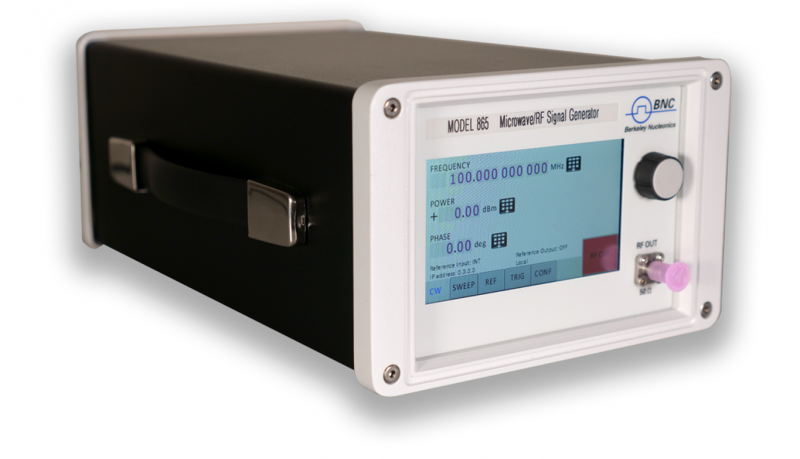
The Model 865B is a low-noise microwave Signal Generator family with continuous coverage from 100 kHz (8 kHz with Option 8K) to 12.75, 20, 26 or 40 GHz depending on model, in 0.001 Hz steps (Figure 3). Its datasheet carries the rows section 3 asks for, and Table 1 collects the phase noise rows at the carrier frequencies a converter clock is likely to use.
| Carrier | 10 Hz offset | 1 kHz offset | 100 kHz offset |
|---|---|---|---|
| 1 GHz | −87 typical; −100 typical with Option LN | −130 typical, −125 maximum | −148 typical, −144 maximum |
| 4 GHz | −74 typical, −68 maximum; −86 typical, −74 maximum with Option LN | −118 typical, −114 maximum | −136 typical, −132 maximum |
| 10 GHz | −67 typical, −60 maximum; −78 typical, −66 maximum with Option LN | −108 typical, −104 maximum | −127 typical, −123 maximum |
| 40 GHz | −55 typical, −48 maximum; −66 typical, −53 maximum with Option LN | −96 typical, −92 maximum | −115 typical, −111 maximum |
Table 1. Model 865B single-sideband phase noise in dBc/Hz from the datasheet, warranted at 23 ±5 °C after a 30 minute warm-up. The rise from 1 GHz to 10 GHz at 1 kHz offset is 22 dB against the 20 dB that pure multiplication would give.
The worked integration. Take the typical 1 GHz row with the standard reference: −87 dBc/Hz at 10 Hz, −130 at 1 kHz and −148 at 100 kHz, joined on log-linear segments as Figure 4 shows. The first segment falls 43 dB over two decades, 21.5 dB per decade, so with m/10 + 1 = −1.15 its integral is 10−8.7 × 10 × [(100)−1.15 − 1] / (−1.15) = 1.73 × 10⁻⁸. The second falls 18 dB over two decades, 9 dB per decade, and integrates to 10−13 × 1000 × [(100)0.1 − 1] / 0.1 = 5.85 × 10⁻¹⁰. The sum is 1.785 × 10⁻⁸, and with the factor 2 of equation (2) the mean-square phase is 3.57 × 10⁻⁸ rad2, so φrms = 1.89 × 10⁻⁴ rad, or 0.0108 degrees. Equation (3) at 1 GHz gives tj = 1.89 × 10⁻⁴ / (2π × 109) = 30.1 fs over 10 Hz to 100 kHz.
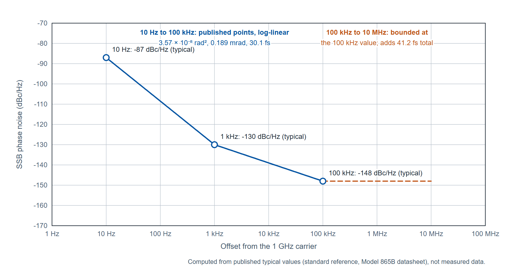
The datasheet tabulates no value above 100 kHz, and a converter integrates well beyond it, so the band from 100 kHz to 10 MHz is bounded rather than computed: on the condition that the noise there is no higher than its 100 kHz value, it contributes at most 10−14.8 × (107 − 105) = 1.57 × 10⁻⁸, almost as much as everything close in. The bounded total is 3.35 × 10⁻⁸, giving φrms = 2.59 × 10⁻⁴ rad and tj = 41.2 fs over 10 Hz to 10 MHz. Put through equation (1), 41.2 fs holds a 1 GHz input to 71.7 dB and a 500 MHz input to 77.8 dB; the 30.1 fs of the published band alone holds 1 GHz to 74.5 dB. The datasheet's phase noise plot carries the curve beyond 100 kHz, and a measured trace on the clock (section 6) replaces the bound with a number.
Three things in that arithmetic are worth more than the result. The 10 Hz to 1 kHz segment supplies 97 percent of the published-band sum, so the lower limit decides the number: starting the integration at 100 Hz instead of 10 Hz gives 9.4 fs from the same table. Option LN changes only the close-in row, from −87 to −100 dBc/Hz at 10 Hz, and that alone brings the 10 Hz to 100 kHz figure from 30.1 fs to 11.0 fs. And a worst-case budget is built from the warranted maxima where the table carries them: with −125 and −144 dBc/Hz in place of the typical −130 and −148, the published band integrates to 34.5 fs and the bounded total to 56.4 fs, which holds a 1 GHz input to 69.0 dB.
Spectral purity. Table 2 carries the rows that set the spur floor, all at 0 dBm output power. By the relation in section 3, the −92 dBc typical non-harmonic figure for carriers between 1.2 and 2.5 GHz, which applies at offsets above 10 kHz, allows output spurs at −92 dBc for an input at the clock frequency and at −112 dBc for an input a decade below it; the warranted maximum of −60 dBc in the same band is the figure for a worst-case budget.
| Quantity (at 0 dBm output) | Condition | Typical | Maximum |
|---|---|---|---|
| Harmonics | 0.01 to 6 GHz | −40 dBc | −30 dBc |
| Harmonics | above 6 GHz | −35 dBc | −30 dBc |
| Harmonics | above 10.5 GHz, 865B-12 and 865B-20 | −55 dBc | −45 dBc |
| Harmonics | above 10.5 GHz, 865B-26 and 865B-40 | −30 dBc | −25 dBc |
| Harmonics | Option FILT, above 20 GHz | −60 dBc | −48 dBc |
| Sub-harmonics | below 5 GHz | −75 dBc | −65 dBc |
| Sub-harmonics | 5 to 20 GHz | −70 dBc | −60 dBc |
| Sub-harmonics | above 20 GHz; with Option FILT | −55 dBc; −65 dBc | −50 dBc; −55 dBc |
| Non-harmonic spurious, offsets above 10 kHz | below 1.2 GHz | −90 dBc | −60 dBc |
| Non-harmonic spurious, offsets above 10 kHz | 1.2 to 2.5 GHz | −92 dBc | −60 dBc |
| Non-harmonic spurious, offsets above 10 kHz | 2.5 to 5 GHz | −90 dBc | −58 dBc |
| Non-harmonic spurious, offsets above 10 kHz | 5 to 10 GHz | −84 dBc | −58 dBc |
| Non-harmonic spurious, offsets above 10 kHz | 10 to 20 GHz | −80 dBc | −58 dBc |
| Non-harmonic spurious, offsets above 10 kHz | above 20 GHz | −70 dBc | −50 dBc |
Table 2. Model 865B spectral purity rows from the datasheet. The harmonic figures with Option FILT below 20 GHz are given by the datasheet's harmonic plots rather than a table row; Option FILT also lowers the maximum output power (section 5).
55. Output power, cable loss and the reference
Table 3 lists the maximum settable output power by band. The old form of this note stated these rows correctly, and they are unchanged here. A clock input with a specified drive range is reached through the cable, and the loss is set by the clock frequency rather than the signal frequency. As an illustration with an assumed cable figure, a flexible coaxial assembly rated at 1.2 dB per meter at 5 GHz loses 3.6 dB over 3 m, so a 5 GHz clock set at the 865B-12 or 865B-20 maximum of +26 dBm arrives at +22.4 dBm; the cable's own datasheet supplies the real figure. For low drive levels the step attenuator options extend the range downward: Option PE4 is an electrical step attenuator to −55 dBm on the 865B-40, and Options PE and PE2 are mechanical step attenuators to −90 and −120 dBm. Level uncertainty below 6 GHz is 0.8 dB maximum (0.25 dB typical) from maximum power down to −15 dBm, rising to 1.2 dB maximum (0.4 dB typical) between 26 and 40 GHz.
| Band | 865B-12 and 865B-20 | 865B-40 | Any model with Option FILT |
|---|---|---|---|
| 8 to 100 kHz (Option 8K) | +15 dBm | +15 dBm | see plot |
| 0.1 to 10 MHz | +24 dBm | +24 dBm | +15 dBm |
| 0.01 to 5 GHz | +26 dBm | +25 dBm (to 6 GHz) | +13 dBm (0.01 to 20 GHz) |
| 5 to 12.75 GHz | +24 dBm | +24 dBm (6 to 12.75 GHz) | +13 dBm |
| 12.75 to 18 GHz | +22 dBm | +21 dBm (12.75 to 26 GHz) | +13 dBm |
| 18 to 20 GHz | +20 dBm | +21 dBm | +13 dBm |
| 26 to 40 GHz | not covered | +18 dBm | +10 dBm (20 to 40 GHz) |
Table 3. Maximum output power by band from the Model 865B datasheet, standard configuration and with Option FILT; the settable minimum is −25 dBm without an attenuator option. Option FILT and the electrical attenuator Option PE4 cannot be combined.
The reference. The internal 100 MHz oven-controlled reference holds ±100 ppb from 0 to 50 °C (±20 ppb with Option LN) and ages 1 ppm in the first year (0.03 ppm with Option LN, 0.02 ppm with Option LN+), and 5 ppb per day after 30 days of operation (0.5 ppb with Option LN). At a 1 GHz clock those figures are 100 Hz over temperature and 1 kHz over the first year. Locking the instrument to the bench reference removes them from the budget: the rear-panel reference input accepts 10 MHz at −5 to +10 dBm with a ±1.5 ppm lock range, integer-megahertz references from 5 to 250 MHz with Option VREF, and a 100 MHz bypass input at +5 to +15 dBm that drives the synthesis directly. The reference output delivers 100 MHz (10 or 100 MHz with Option LN) at 0 dBm for the rest of the bench. Switching takes 1.5 ms from a SCPI CW command, 500 µs per point in list mode and 30 µs with Option FS; control is by SCPI 1999 over LAN, USB 2.0 or optional GPIB, from the front-panel touch display, or from the browser interface the instrument serves. The chassis is 4.21 in high, 6.77 in wide and 11.42 in deep at 2.5 kg, with Option RM for a 3U rack kit and Option 1URM for a 1U rack module.
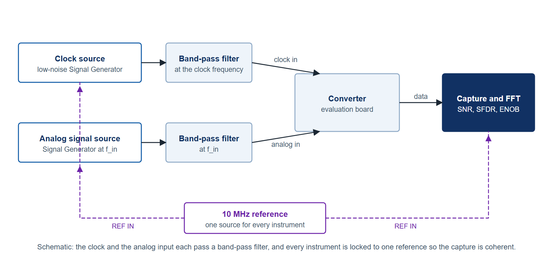
When the clock and the test tone come from one chassis. A converter test needs an analog input as well as a clock, and Figure 5 shows the setup with the two sources separate and locked to one reference. Where the two signals have to come from a single unit, the Model 865B-M-X is the instrument for that job: a 19 in, 1U synthesizer with one to four fully independent outputs, each settable in frequency, power, phase and modulation from 100 kHz (8 kHz with Option 8K) to 40 GHz, sharing one internal oven-controlled reference, with a published typical phase noise of −130 dBc/Hz at 1 kHz from a 1 GHz carrier and a wideband floor of −160 dBc/Hz, and with units cascadable on one master reference clock for phase coherence across chassis.
66. Measurement practice
These steps apply to any clock source and any converter, and none of them requires buying an instrument.
- Share one reference. Lock the clock source, the signal source and the capture system to a single 10 MHz (or 100 MHz) reference, and choose the input frequency so that an integer number of input cycles fits the capture record. Coherent sampling removes the window leakage that otherwise hides the noise floor and the spurs the clock produces.
- Filter the clock. A band-pass filter at the clock frequency, placed at the converter end of the cable, removes the source's harmonics and far-out noise before the clock receiver. The filter's bandwidth is the upper limit of the jitter integration: a 10 MHz filter bandwidth is the 10 MHz upper limit in section 4.
- Set the slew rate deliberately. A clock receiver converts the amplitude noise present at its threshold into timing noise in inverse proportion to the slope of the edge:
where vn is the rms noise voltage at the receiver threshold within its bandwidth (100 µV is used below as an illustrative assumption, not a specification) and dv/dt is the slope of the clock at the threshold crossing, 2πf0Vpk for a sine of peak voltage Vpk.
A +10 dBm sine into 50 Ω has a peak of 1.00 V and, at 1 GHz, a zero-crossing slope of 6.28 V/ns; with the assumed 100 µV of threshold noise, equation (4) gives 15.9 fs. At 0 dBm the peak is 0.316 V, the slope is 1.99 V/ns and the same noise gives 50.3 fs, and at +20 dBm the figures are 3.16 V, 19.9 V/ns and 5.0 fs. The drive level is therefore part of the jitter budget, within the converter's absolute maximum ratings, which is why a source that delivers +26 dBm below 5 GHz with a stated level accuracy is useful here: the slope can be set and known.
- Route the clock away from the signal. Keep the clock cable, the analog input cable and the data lines physically separated; a clock harmonic coupled into the analog input appears as a spur that no clock specification predicts.
- Measure the clock where it is used. A two-channel cross-correlation phase noise analyzer such as the 7000 Series measures the clock at the converter's clock connector, filter and cable included, and reports the integrated rms phase deviation and time jitter over a band you set. That measurement replaces the bound in section 4 with a number and separates the clock's contribution from the converter's own aperture jitter.
- Record the band with the number. Every jitter figure in the test report carries its lower and upper offset limits, the clock frequency, the drive level and the filter, so a later measurement can be compared with it.
77. Limitations
The worked figures in section 4 use typical values, which the datasheet defines as expected mean values rather than warranted performance; a budget that has to survive a production floor is built from the warranted maxima, as the 34.5 fs and 56.4 fs figures show. The 100 kHz to 10 MHz band is bounded on an assumption, not computed from a table, and only the datasheet plot or a measured trace settles it. The 10 Hz value at 1 GHz is carried as typical only, for the standard and the Option LN reference.
Option FILT improves the harmonic rows at a cost: the maximum output falls to +13 dBm from 0.01 to 20 GHz and +10 dBm from 20 to 40 GHz, and the option cannot be combined with the electrical step attenuator Option PE4. The slope argument of equation (4) then limits how low the threshold noise contribution can be driven.
A converter with an internal phase-locked loop that multiplies a low-frequency reference adds its own jitter inside the loop bandwidth, and nothing in the clock source changes that term; the measurement of step 5 shows which side of the connector a problem is on.
You may not need this instrument. A 12-bit converter with a 100 MHz input tolerates 318 fs, and a 14-bit converter 80 fs, which a good crystal-oscillator clock with a band-pass filter can meet. The case for a low-noise microwave Signal Generator is a gigahertz-class input at 12 bits or more, a test that has to sweep the clock frequency, or a bench where the clock, the test signal and the capture must share one reference and one control interface.
8Summary
| Quantity | Value | Condition |
|---|---|---|
| Jitter-limited SNR | −20 log10(2πfintj) | Equation (1); full-scale sine input, converter otherwise ideal |
| Jitter for the 12-bit ideal (74.0 dB) | 31.8 fs at 1 GHz input; 318 fs at 100 MHz | From equation (1) |
| Jitter for the 14-bit ideal (86.0 dB) | 8.0 fs at 1 GHz input; 80 fs at 100 MHz | From equation (1) |
| Model 865B, 1 GHz, 10 Hz to 100 kHz | 30.1 fs rms (0.0108 degrees) | Typical values, standard reference, log-linear segments |
| Model 865B, 1 GHz, 10 Hz to 10 MHz | 41.2 fs rms | Typical values; 100 kHz to 10 MHz bounded at the 100 kHz value |
| Same, Option LN, 10 Hz to 100 kHz | 11.0 fs rms | −100 dBc/Hz typical at 10 Hz in place of −87 |
| Same, warranted maxima at 1 kHz and 100 kHz | 34.5 fs (published band); 56.4 fs (bounded to 10 MHz) | −125 and −144 dBc/Hz; 10 Hz typical |
| Output spur from a clock spur | clock spur level + 20 log10(fin/fclk) | Small phase-modulation spur |
| Reference stability at 1 GHz | 100 Hz over 0 to 50 °C; 1 kHz first-year aging | Standard reference; 20 Hz and 30 Hz with Option LN |
9Definitions
Aperture jitter. The random variation of the instant at which a converter samples its input, expressed as an rms time.
Coherent sampling. Choosing the input frequency, sample rate and record length so that an integer number of input cycles fits the record, with every instrument on one reference, so that the transform needs no window.
Integrated phase noise. The mean-square (or rms) phase deviation obtained by integrating the single-sideband phase noise over a stated offset band, equation (2).
Non-harmonic spurious. A discrete output component that is neither a harmonic nor a sub-harmonic of the carrier, stated as a level relative to the carrier at offsets beyond a stated minimum.
Single-sideband phase noise, L(f). The ratio of the power in one phase-modulation sideband, in a 1 Hz bandwidth at offset f from the carrier, to the total carrier power, expressed in dBc/Hz (IEEE Std 1139).
Slew rate. The rate of change of voltage with time at a point on a waveform, in volts per second; for a sine at the zero crossing, 2πf0Vpk.
Sub-harmonic. A discrete output component at a sub-multiple of the carrier frequency, produced by the frequency multiplication inside a synthesizer.
Typical and maximum. On the Model 865B datasheet, typical values are expected mean values and not warranted performance; minimum and maximum values are guaranteed by design or production test with guard bands, at 23 ±5 °C after a 30 minute warm-up.
10Symbols
| Symbol | Meaning | Unit |
|---|---|---|
| A | Peak amplitude of the converter input | V |
| fin | Converter input frequency | Hz |
| f0, fclk | Clock (carrier) frequency | Hz |
| f1, f2 | Lower and upper offset limits of the integration | Hz |
| fs | Offset of a spur from the clock | Hz |
| L(f) | Single-sideband phase noise at offset f | dBc/Hz, or a power ratio per hertz |
| m | Slope of a log-linear phase noise segment | dB per decade |
| N | Converter resolution | bits |
| tj | rms clock jitter over the stated band | s |
| vn | rms noise voltage at the clock receiver threshold | V |
| Vpk | Peak voltage of the clock sine | V |
| φrms | rms phase deviation over the stated band | rad |
11Acronyms
ADC, analog-to-digital converter. CW, continuous wave. DAC, digital-to-analog converter. ENOB, effective number of bits. FFT, fast Fourier transform. GPIB, general purpose interface bus. LAN, local area network. OCXO, oven-controlled crystal oscillator. ppb, parts per billion. ppm, parts per million. rms, root mean square. SCPI, Standard Commands for Programmable Instruments. SFDR, spurious-free dynamic range. SNR, signal-to-noise ratio. SSB, single sideband. USB, universal serial bus.
12Further reading
- Model 865B datasheet, the specification source for every value in this note: web edition and PDF.
- Model 865B-M-X multi-channel synthesizer datasheet: web edition and PDF.
- 7000 Series phase noise analyzer datasheet, for measuring a clock at its connector: web edition and PDF.
- Berkeley Nucleonics technical notes: Phase noise and spectral purity in RF Signal Generators, Phase noise measurement basics and Measuring a 100 MHz OCXO with cross-correlation.
- IEEE Std 1139-2008, IEEE Standard Definitions of Physical Quantities for Fundamental Frequency and Time Metrology, Random Instabilities. doi:10.1109/IEEESTD.2008.4797525.
- IEEE Std 1241-2010, IEEE Standard for Terminology and Test Methods for Analog-to-Digital Converters. doi:10.1109/IEEESTD.2011.5692956.
13Discuss your clock requirement
Our application engineers would be glad to work through a jitter budget for a specific converter and band with you, or to arrange a demonstration of the Model 865B on your bench. Request a quote or demo, write to info@berkeleynucleonics.com, or call 800-234-7858.