 Powered by Bioz
§Warranty
Berkeley Nucleonics shall not be responsible for defects caused by natural wear and tear, willful damage, negligence, force majeure, abnormal working conditions, or failure to follow Berkeley Nucleonics spoken or written guidelines as to the storage, installation, commissioning, use, or maintenance of the products or (if there are none) good trade practice; or where the customer alters or repairs such goods without written consent from Berkeley Nucleonics. Opening the instrument and/or breaking warranty seals voids the warranty. Service plans are subject to the same warranty policy regarding use.
Copyright
This manual is copyright by Berkeley Nucleonics and all rights are reserved. No portion of this document may be reproduced, copied, transmitted, transcribed, stored in a retrieval system, or translated in any form or by any means such as electronic, mechanical, magnetic, optical, chemical, manual, or otherwise, without written permission of Berkeley Nucleonics.
General Warranty
Warranty is 1 Year standard, unless otherwise specified. Materials and workmanship, return to manufacturer included.
If the product proves defective during the warranty period, Berkeley Nucleonics either will repair the defective product without charge for parts and labor or will provide a replacement in exchange for the defective product. Parts, modules, and replacement products used by Berkeley Nucleonics for warranty work may be new or reconditioned to like-new performance. All replaced parts, modules, and products become the property of Berkeley Nucleonics.
To obtain service under this warranty, the Customer must notify Berkeley Nucleonics of the defect before the expiration of the warranty period. The Customer shall be responsible for packaging and shipping the defective product to the service center designated by Berkeley Nucleonics, along with a copy of customer proof of purchase.
This warranty shall not apply to any defect, failure, or damage caused by improper use or by improper or inadequate maintenance and care. Berkeley Nucleonics shall not be obligated to furnish service under this warranty:
- a) to repair damage resulting from attempts by personnel other than Berkeley Nucleonics representatives to install, repair, or service the product;
- b) to repair damage resulting from improper use or connection to incompatible equipment;
- c) to repair any damage or malfunction caused by the use of non-Berkeley Nucleonics supplies; or
- d) to service a product that has been modified or integrated with other products when the effect of such modification or integration increases the time or difficulty of servicing the product.
1Introduction & Notices
Notices
©2023 Berkeley Nucleonics Corp. This document contains information which is copyright protected. No part of this manual may be reproduced in any form without prior agreed written permission from Berkeley Nucleonics Corporation as governed by United States and International copyright laws.
- WARNING indicates a potential hazard that could completely damage the product. Do not continue until you fully understand the meaning.
- CAUTION indicates a potential hazard that could partially damage the product. Do not continue until you fully understand the meaning.
- NOTE provides additional pertinent information related to the operation of the product.
The information contained in this document is subject to change without notice. There is no guarantee as to the accuracy of the material presented or its application. Any errors of commission or omission will be corrected in subsequent revisions or made available by errata. Refer to the product specification sheet or the Berkeley Nucleonics website for warranty information on the specific product of interest. Document number: not assigned (reference the Model 12100 Series product manual for the PowerEye Precision Power Meter application).
What Is Covered in This Manual
This manual covers installation and operation of the Model 12100 Series USB power sensors using PowerEye Precision Power Meter software, which make True RMS Average (CW or modulated) measurements. It also covers product features and support, specifications, compatibility, and measurement examples. Refer to the sensor's Programming Manual for programmatic remote control information.
The Model 12175 is part of the Model 12100 Series and is supported by the PowerEye operating procedures described in this manual. Sensor-specific specifications, including frequency and power range, are provided in the current Model 12100 Series datasheet.
- Section 1 covers general information and installation.
- Section 2 discusses various measurements and how to make them.
- Section 3 explains the menus, features, and functions of PowerEye, and how to access them.
Additional documentation and support is available from Berkeley Nucleonics: a detailed Programming Guide, a Programmatic Measurement Examples Guide, an SPI and I2C Interface User's Guide, Interactive IO Control software, programmatic example code, and drivers and support for LabVIEW and other environments.
Overview
The Model 12100 Series USB Power Sensor is a compact power sensor body that connects directly to a desktop or laptop computer over a standard USB 2 port. The sensor converts RF and microwave power into fully calibrated, processed digital data. The companion PowerEye Precision Power Meter software provides a front-panel display for typical average power measurements as well as advanced triggered, time-gated measurements.
The Model 12175 extends the Model 12100 Series frequency coverage to 50 GHz to 75 GHz. It uses a WR-15 waveguide RF input and has a specified operating range of -50 dBm to +18 dBm. Operation through PowerEye follows the same general workflow described throughout this guide.
Sensor-specific specifications are detailed in the Model 12100 Series datasheet; programmatic information is covered in the Model 12100 Programming Guide.
Patented No-Zero No-Cal features eliminate sensor zeroing and meter reference calibration. The sensor features optional Trigger IN/OUT or Recorder OUT connectors in addition to the model's RF input interface; see the datasheet for the complete option list.
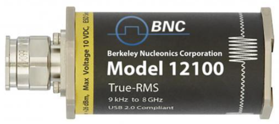
Sensors Compatible with PowerEye Software
All Model 12100 Series sensors are compatible with PowerEye software; portions of the application are sensitive to the sensor's firmware version and purchased options. In some cases the sensor's firmware may require updating to use the latest PowerEye version, in which case PowerEye issues a warning and may close — send the sensor back to Berkeley Nucleonics for updating. Earlier software versions are also available from Berkeley Nucleonics sales.
Use of Multiple Sensors
PowerEye is a multi-threaded application capable of reliably controlling 12 or more individual Model 12100 sensors at one time, each controlled by its own sensor window. A two-sensor calculation window with various derived functions is also included; see Derived Measurements in Section 2.
Windows Versions (PowerEye Software)
PowerEye and the included Interactive IO are Windows-based, compatible with Windows XP through the latest Windows version, 32- and 64-bit, and use the computer's native USB HID system driver.
Interface Description (Sensor)
Model 12100 Series sensors are composite USB devices with both USBTMC and USB HID interfaces, plus optional SPI and I2C interfaces. The USB HID interface loads when a sensor is connected to Windows, LINUX, Apple, or other computers with standard USB HID interfaces.
Important Interface Notes
- USBTMC driver. A connected computer may attempt to load a USBTMC driver; if you don't intend to use USBTMC, ignore the error.
- Device Manager warning. A missing-driver warning in Windows Device Manager is normal if USBTMC is not present on the computer, and is harmless.
- Option SPI. Sensors with Option SPI (SPI and I2C interfaces) also include fully functioning USB ports. Do not use the USB port while the SPI/I2C port is in use, or vice versa.
LINUX
Linux-based computers, like most PCs, have native USB HID drivers, and the Model 12100 sensor loads this native driver when connected. PowerEye software itself is Windows-based; contact Berkeley Nucleonics sales to discuss LINUX support.
Programming Guide Utilization
A complete detailed programming guide is available on the Berkeley Nucleonics website. PowerEye uses the commands detailed in the guide to make measurements; advanced users are encouraged to review the guide for a full understanding of measurement nuances — for example, the DCYC or GAINx offset commands behind PowerEye's simple offset feature.
Installation
Insert the flash drive or open the download link from Berkeley Nucleonics. If install does not start automatically, run setup.exe; installation is automatic. If the installer requests a driver from the internet, answer no or ignore — PowerEye uses default system drivers and no additional drivers are required. Leave the Interactive I/O application selected if you plan to test programmatic commands. Refer to the quick start card for other install details.
2Making Measurements
Your First Measurement
With the sensor connected, locate PowerEye in the Berkeley Nucleonics Technologies folder and start the program. After a few seconds the software and sensor are running; by default three windows open — the main Sensor Window, an Analog Meter, and a Strip Chart.
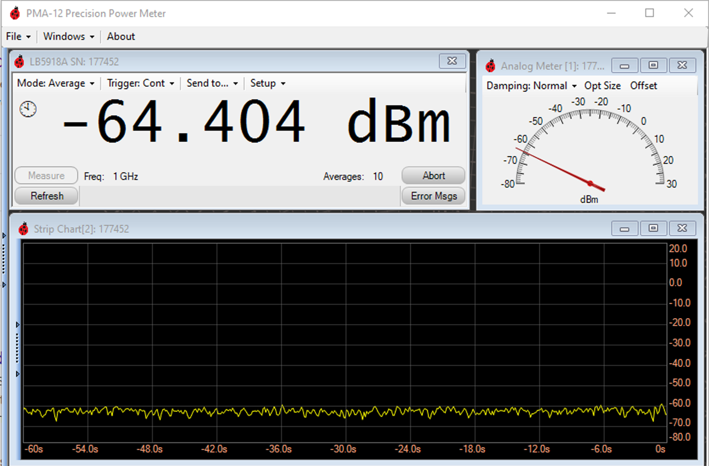
The Sensor Window is the primary control for the sensor and the measurement; it is the only window communicating with the sensor. Closing it terminates the sensor connection, though the Strip Chart and Logs remain open with their already-collected data — the sensor can be reopened from the details pane or by restarting the application. The Analog Meter simply displays data collected by the Sensor Window and can be closed if not needed. The Strip Chart graphically shows signal changes and is useful, for example, when determining how much averaging is needed for a clean, accurate measurement.
As with any power measurement, a few important parameters must be set. Connect the RF source or DUT to the sensor RF input; for the Model 12175, connect through the WR-15 waveguide interface. Once connected, set PowerEye to the actual measurement frequency of the applied signal.
Frequency
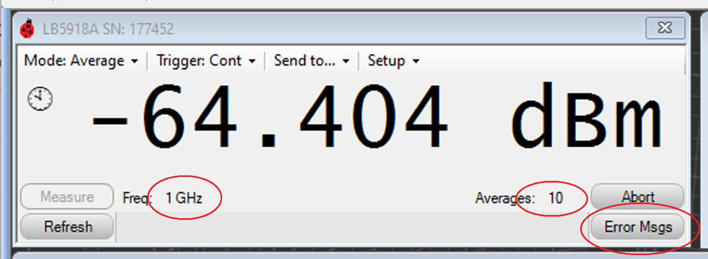
Power sensors are calibrated at various frequencies to achieve high accuracy. Click the displayed frequency and set your signal's frequency so the sensor applies the appropriate calibration data. Screen images and worked examples elsewhere in this guide may show representative frequencies; use the actual measurement frequency for the sensor in use.
Averages
The power sensor collects readings and averages them together; the number of Averages sets how much time is collected before a measurement becomes available (also called the capture time). With PowerEye's defaults, each measurement takes about 250 ms. Reasons to adjust it:
- Long PRT. For a signal with a long time between pulses, such as radar, increase averages (over 1,000 is possible) to include many pulses.
- Low signal level. Increase averages to mitigate noise on a very low-power signal.
- High resolution. With sufficient power and a clean signal, reduce averages to see signal changes more quickly on the strip chart or tabular log.
Error Reporting
The Model 12100 Series sensors maintain an internal error log compliant with IVI SCPI instrument standards. The sensor issues an error for reasons including an out-of-range parameter, a communication error, or an interruption while processing a command or query — for example, setting a parameter while the sensor is mid-measurement, a harmless, accidental error reported by a red sensor LED. Click Error Msgs in PowerEye to request, clear, and display the sensor's error messages.
Advanced Measurements & Features
This section is not intended to cover every capability of the sensor and PowerEye software; details on accessing the menus and features referenced below are in Section 3. Reference to the Programming Guide is also encouraged.
Measurement Timing
An average is made up of processed and calibrated readings. By default, PowerEye sets the sensor's rate for each individual reading to 40 per second (MRATe in the programming guide). With Averages set to 10, each measurement consists of 10 averages / 40 readings per second, or ¼ second — the capture time. This is the rate the sensor itself makes the measurement, not necessarily the rate PowerEye displays it.
Measurement Latency. PowerEye requests measurements from the sensor, and the sensor processes the request as above. Because this is typically faster than can be visualized, a delay called Measurement Latency is added between requests, set in the Trigger dropdown menu. By default PowerEye uses the FETCh? query, so the sensor free-runs and PowerEye receives the measurement as soon as it requests it. If Display Update Mode is set to Upon Completed Measurement, the READ? query is used instead, and the measurement begins when PowerEye requests it.
Intermediate Results. At startup, with Display Update Mode set to Intermediate Results, the sensor is free-running and PowerEye simply requests a measurement; the sensor immediately returns the last 10 averages (default). This is a "trailing" measurement, similar to a thermal sensor, reporting the power level just before the display shows it.
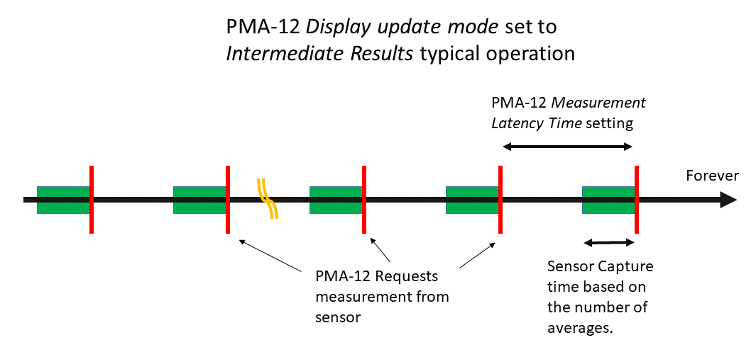
If the number of averages is changed so a long period is captured, the display may show an intermediate result before all averages are collected — this only matters when the capture time is very long compared to the display update rate. A circular buffer means that once a complete set of averages is collected, the measurement uses the most recent set.
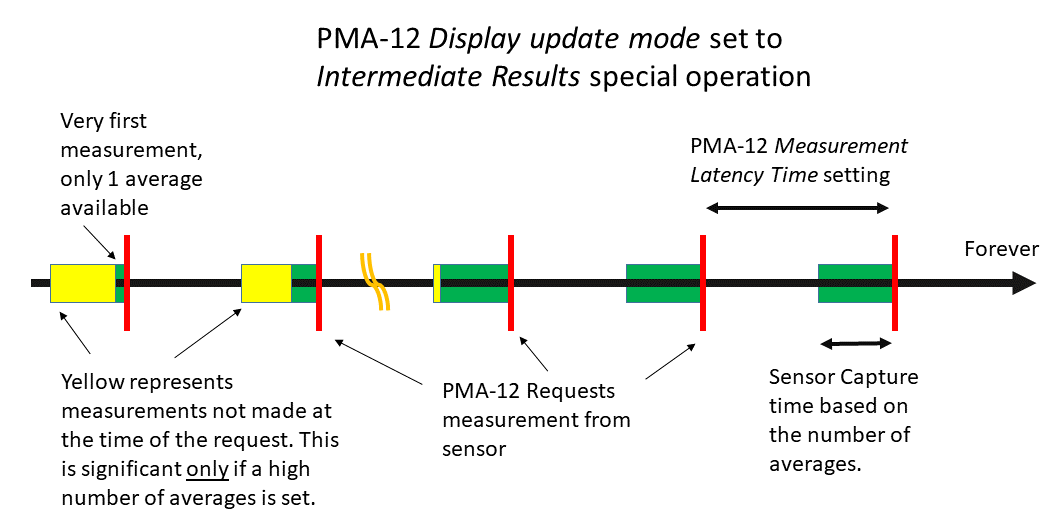
Upon Completed Measurement. With Display Update Mode set to Upon Completed Measurement, the sensor's READ? query starts a new measurement with fresh readings each time — ideal whenever the measurement start time matters, and useful for triggered measurements, which normally define the start of a capture.
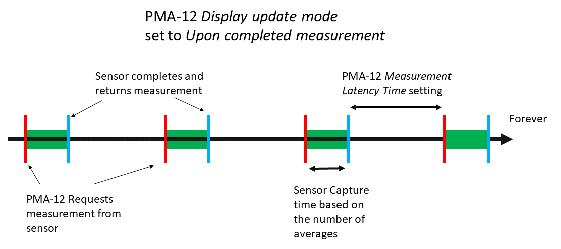
Typical users viewing a signal graphically may not notice the timing difference between Intermediate Results and Upon Completed Measurement, since measurements occur in milliseconds; the distinction matters most to programmatic users and anyone using triggering.
Simulated Sensors
Simulated sensors are available from the Details Pane: Open/Close, then Simulated Sensor. A simulated sensor is used in the Derived Measurements example below.
Derived Measurements
PowerEye can calculate a measurement between two sensors, from the Derived Measurements window: Reflection Coefficient, VSWR, Return Loss, Mismatch Loss, Gain, or Loss.
Example gain measurement on a module, using an active sensor and a simulated sensor standing in for a 20 dB input coupler terminated into a sensor:
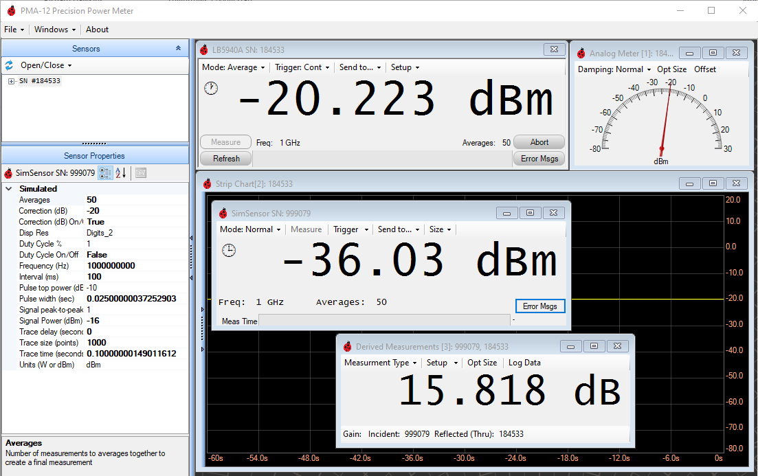
- Start PowerEye and set the frequency.
- Apply power to the actual sensor.
- Open the simulated sensor and, in its Details Pane, set the power to -56 dBm plus a 20 dB correction for the coupler, and enable it.
- Open a Derived Measurement window, set Measurement Type to Gain, and in Setup set the Incident sensor to the simulated sensor and the actual sensor to Thru.
- Increase averages to 50 on both sensors for stability.
The example result shows the module has a positive gain of 15 dB — the same setup works with two real sensors for a real-world measurement.
Saving Derived Measurement Data. Select Log Data in the Derived Measurements window to open a logger that automatically stores data. To save, Pause the logger, then File > Save opens a standard Windows file dialog; the saved file opens in Excel or another compatible tool. While paused, data can also be selected and copied to the clipboard. Data can be stored while paused (the default), set from the logger's Options dropdown.
Triggered Measurements
This covers external triggering in the default Average Mode using the READ? query (see Trace Measurements below for triggered measurements in trace mode). Consider: capture time, external triggering, single vs. continuous measurements, and whether delay or pre-trigger data is required.
Worked example: a 1 GHz signal with 150 ms on-time, repetitive with a 500 ms PRT. Worked examples throughout this guide may use representative Model 12100 Series settings; when following these procedures, set the frequency to the actual signal frequency supported by the connected sensor.
- Trigger dropdown: set triggering to Single (so setup commands aren't sent), Display Update Mode to Upon Completed Measurement (so READ? is used), and Trigger Source to External.
- Capture time: to capture about 100 ms of on-time (video rise time in Average mode is about 7 ms), and with MRATe doubled at startup (25 ms/average), 100 ms ÷ 25 ms = 4 — set Averages to 4.
- External TTL triggering is used here; internal triggering is not available in Average mode (it returns a settings-conflict error) — internal triggering is available in trace mode.
- Trigger section (Details Pane): set Slope to Positive (trigger on rising input) and Trig Delay to 10 ms to account for the sensor's video rise time.
Set frequency to 1 GHz, turn on the RF source and external trigger, then set Trigger to Continuous (or Single, to try individual manual measurements — the Measure button highlights and clicking it initiates a measurement, after which the sensor waits for a trigger). In Continuous mode, PowerEye automatically initiates a measurement per the Measurement Latency time.
Locating Minimum and Maximum Power
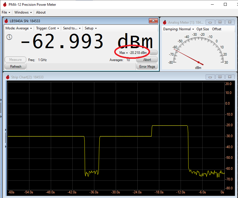
PowerEye can automatically monitor, locate, and report the lowest and highest power level. From the Sensor Window, select Setup, then Min Hold or Max Hold; the value appears in the lower right of the sensor window. The small button beside the value resets the measurement to a new starting value.
Displaying Relative Power
Relative Power (labeled Rel, in the same lower-right location as Min/Max Hold) shows the power between a pre-set level and the current power. Click the small oval beside the value to reset the compare value to the current value.
Frequency Dependent Offsets
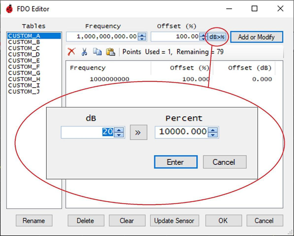
Model 12100 sensors carry 10 internal Frequency Dependent Offset (FDO) tables, each holding up to 80 offsets, to correct measurements at various frequencies — for example, characterizing an attenuator, coupler, or cable whose response varies slightly over frequency. Using an FDO takes three steps:
- Enter the FDO data into one of the tables (Setup dropdown > FDO Editor).
- Select the table (Setup dropdown > FDO Selection).
- Enable the FDO by setting FDO Enabled to True in the Sense section of the Sensor Properties pane.
The 10 tables and the FDO function live in the sensor itself and are also available to ATE test systems, not just PowerEye.
Simple Offset Correction
A simple offset quickly corrects for an attenuator, coupler, or similar situation where frequency-dependent adjustment isn't needed. In the Details Pane, place the desired value in dB in Correction (dB) and set Correction (dB) Enabled to True. The value is added to the reading (positive or negative) — for example, a 10 dB correction turns a -31.5 dBm reading into -21.5 dBm, or into -41.5 dBm with a -10 dB correction. This function also lives in the sensor itself, available to ATE systems.
Duty Cycle Correction (Pulse Power)
Duty Cycle Correction derives pulse power from average power given a known duty cycle, controlled from the Details Pane: set Averaging so the measurement is stable across many cycles, place the known duty cycle (as a percentage) in Duty Cycle %, and set Duty Cycle Enabled to True. This function also lives in the sensor itself, available to ATE systems.
75 Ohm Measurements
A simple offset specifically for 75 Ω measurements is built in, for use with a standard MLP (Minimum Loss Pad) — a resistive divider presenting 75 Ω to the DUT and 50 Ω to the sensor. An MLP's 5.72 dB loss is pre-programmed into the sensor. Acquire and install an MLP (available from Berkeley Nucleonics), then set MLP Enabled to True in the Details Pane; 5.72 dB is added to the measurement to correct for the MLP. Refer to the sensor-specific datasheet before applying connector-specific accessories.
Trace Measurements
Model 12100 Series sensors have two operating modes tied to the video detector filter and sensor firmware:
- Average Mode (default, not trace) is designed for high-dynamic-range general power measurement. Detected video filter rise time is about 7 ms, improving low-level range down to -60 dBm or below.
- Normal Mode (used with trace) suits a triggered measurement examining power at a specific point in time, or visualizing part of a signal, with a rich triggering feature set including pre-trigger data. The detected video filter is typically 60 kHz with a rise time of about 7 µs. Because the sensor's diodes operate in square law and need analog filtering to reduce noise at low levels, Normal Mode's speed-optimized filter raises the minimum usable power to around -40 dBm.
Trace mode is entered from the Sensor Window's Mode dropdown; PowerEye configures itself and the sensor and a Trace Display appears with its own Control Pane (see Trace Mode Controls in Section 3).
Triggered Trace Measurements. Nearly all trace-mode measurements are triggered when the signal meets set parameters. As a minimum, know: Trigger Level (the power level that causes the trigger), Trigger Polarity (slope/direction of change), Hysteresis (signal level), and Trace Time (the time the sensor collects data, displayed left to right).
Example: a pulse stream at +5 dBm (or off), 500 µs pulse width. Only three changes from defaults were needed — Trigger Level -1 dBm, Hysteresis 2 dB, Trigger Source Internal.
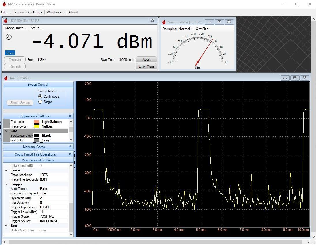
The -4.071 dBm reading in the Sensor Window is the average power of the trace, which may not equal the signal's true average power since the trace may not contain an exact number of complete pulses — increasing Trace Time to include many pulses improves accuracy. The measurement can be refined further: adding a -1 ms trigger delay reveals pre-trigger data, a marker at 1.3 ms, and a gate measuring the average power of one cycle.
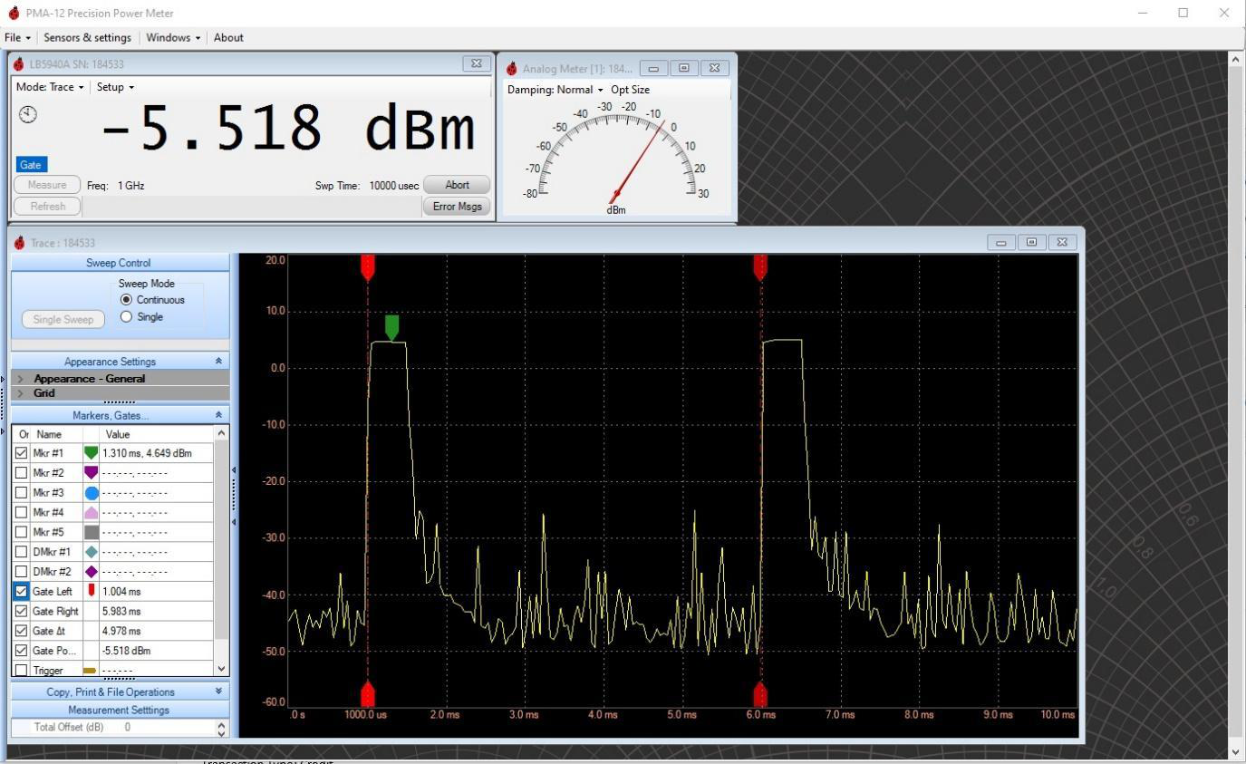
Externally triggered measurements work the same way except the trigger is applied through the sensor's SMB connector; because the trigger is digital, level and hysteresis don't apply, but slope, delay, and impedance still matter. Figures 8 and 9 also represent the same signal with an external trigger and Trigger Source set to External.
Recorder Out (Analog Output)
The Analog Recorder Output (Option 001) is a 0 to 1 VDC output scaled to the measured RF input power. Trigger Out shares its connector with Recorder Out — only one can be used at a time. While in Recorder Out mode, sensor averaging and other standard parameters are forced to the values Recorder Out requires; the display still shows power level, but Sensor Window and Details Pane settings are restricted. PowerEye controls Recorder Out using standard SCPI commands, and programmatic users have full control (see the programming guide). Recorder Out can also run unattended, with no computer attached, once set up — only power is required. A settable filter with broad adjustability can turn low-duty-cycle pulses into a stable analog level representing average power.
Recorder Out Level Settings. Set the power level for 0 V output (Recorder Out Lower) and for 1 V output (Recorder Out Upper) in the Output section of the Details Pane. Power below the lower level yields 0 V; power above the upper level yields 1 V. Output levels depend on proper resistive loading — a 1,000 Ω load (precision resistance recommended) is required to meet the voltage specification. Between the two levels the output is linear.
To determine the output voltage for a given dBm level:
| Symbol | Meaning |
|---|---|
| Vout | (10PMEAS/10 − 10ZeroVoltSet/10) / (10OneVoltSet/10 − 10ZeroVoltSet/10) |
The same formula in Excel, pasted into cell B4 (=(10^(B3/10)-10^(B2/10))/(10^(B1/10)-10^(B2/10))): B1 = dBm setting for 1 V, B2 = dBm setting for 0 V, B3 = desired input power in dBm. All power units are dBm; out-of-range data is not accounted for.
| Power | Recorder Out Low Setting | Recorder Out High Setting | DC Voltage |
|---|---|---|---|
| +10 dBm (10 mW) | -10 dBm (0.1 mW) | +10 dBm (10 mW) | 1 Volt |
| -10 dBm (0.1 mW) | -10 dBm (0.1 mW) | +10 dBm (10 mW) | 0 Volts |
| 0 dBm (1 mW) | -10 dBm (0.1 mW) | +10 dBm (10 mW) | 0.10 Volts |
| -24.4 dBm (3.6 µW) | -40 dBm (0.1 mW) | -20 dBm (10 mW) | 0.37 Volts |
Recorder Out Filter. The digitally applied RO Cutoff Freq (Hz) filter is set in the Output section of the Details Pane. For most Model 12100 Series sensors the default is 32 Hz; the lowest settable frequency is 0.001 Hz.
Recorder Out Activation. Set the Lower and Upper levels and filter as desired, set Mode to Recorder Out in the Sensor Window, then click the Start RO button that appears. Click Halt RO to stop, then select Average in the Mode dropdown.
Grounding and Ground Loops. Model 12100 sensors have solid grounding between the USB shield, USB Common, and SMB (Recorder Out) Common. Consider ground current between connected equipment when using Recorder Out — many USB cables have over an ohm of resistance, and with a 200 mA sensor draw there can easily be 200 mV across the cable; if the computer and the device monitoring Recorder Out share a common ground, this can drive a loop current and create a ground-offset voltage on the monitoring device.
Operation with No Computer Attached. Standard Recorder Out (Option 001) can run with no computer attached, calibrated and scaled per its settings, using the Unattended Operation controls — Option UOP is not required for Recorder Out to work unattended. To use it: set the Upper/Lower levels and filter; in the Basic Unattended Operation section of the Details Pane set UOP Recorder Out Enabled to True; in the Sensor Window Mode dropdown select UOP; in the Start UOP dropdown select Do Not Save Data. The sensor then activates Recorder Out and can be unplugged from the computer and run from a 5.0 V battery or other power source, continuing through power cycles until reconnected to PowerEye and UOP is halted (also available programmatically). To disable, reconnect to a computer running PowerEye — the Sensor Window shows "UOP in progress" — select Halt UOP, then Average in the Mode dropdown.
Unattended Measurements (Unattended Operation)
Option UOP lets the sensor function with no computer connected, using its current measurement setup (frequency and averages) and storing measurements in non-volatile memory. Unattended operation also works while connected to a computer, ensuring measurements aren't interrupted by other USB activity. UOP can store up to 1,000 measurements per second, so its own UOP Latency setting (1 ms to 86,400 seconds) paces storage — a 1 second setting places 1 second between measurements. An optional Timer stops measuring after a set duration (for example, 1 hour) and returns the sensor to normal mode on the next power-up.
Setup and Measure. Verify the clock is set before starting (see Section 3, System). Then: set the measurement frequency and number of averages; in the Trigger dropdown set Display Update Mode to Intermediate Results; in the Mode dropdown select UOP; under Manage UOP set the UOP Measurement Latency (for example 0.1 seconds) and, if desired, the UOP Timer with Enable UOP Timer; in the Start UOP dropdown click Save Data. The sensor begins measuring; disconnect it from the computer and connect it to a 5.0 V source to continue measuring and storing unattended.
Retrieve UOP Data. Data is stored in the sensor's non-volatile memory (check the datasheet for memory depth) as records of index, date, time, value in dBm, and a flags field.
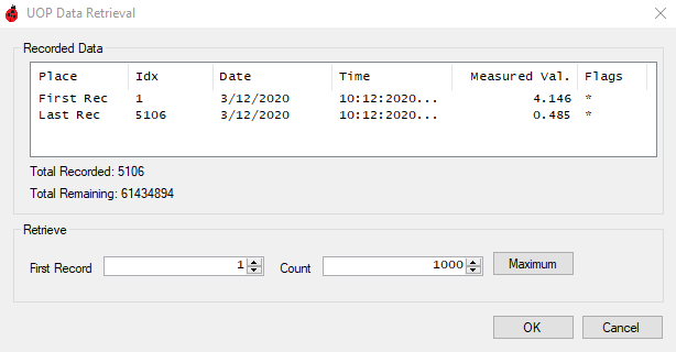
To retrieve: connect to the computer and open the sensor if it doesn't open automatically (the "UOP In Progress…" screen appears while the sensor keeps storing); click Halt UOP to stop; from the Manage UOP dropdown click Retrieve Data; click Maximum to download all measurements, or set First Record and Count to select a specific range. Once the UOP Log appears, the File dropdown offers the standard PowerEye analysis features (Strip Chart and more), and the data can be saved for Excel or other tools.
3Accessing Menus & Features
PowerEye Controls — Sensor Window
Four dropdown menus at the top of the Sensor Window control the measurement. Most settings send commands that change sensor behavior; a few change only PowerEye's own software settings.
Mode Dropdown
Controls presets, Unattended Operation (optional), Recorder Out (optional), and the two basic measurement types, Average and Trace.
- Average — the sensor's default mode, collecting and averaging samples into the displayed measurement.
- Preset Average — a safety net that returns PowerEye and the sensor to startup settings.
- User Preset — loads (recalls) a saved User Preset's parameters.
- Configure User Preset — saves current settings as a preset to load later, or sets them to load automatically at startup (useful in manufacturing); user presets can also be cleared here.
- UOP — on sensors with the optional Unattended Operation feature, places PowerEye and the sensor in Unattended Mode.
- Recorder Out — on sensors with the optional Recorder Out feature, places PowerEye and the sensor in Recorder Out Mode; many settings (such as averages) are then forced and cannot be changed.
- Trace — on sensors with trace capability, switches PowerEye to a time-domain display similar to the Strip Chart but at the sensor's maximum sampling rate, each sample fully calibrated and un-averaged; the sensor's hardware filter changes to ±60 kHz.
- Close Sensor — closes the sensor window and disconnects the sensor driver.
Trigger Dropdown
Controls measurement and display timing plus internal/external triggering; some related settings (such as trigger level) live in the Details Pane.
- Continuous & Single. Continuous (default) sets the sensor to free-run (INIT:CONT ON, trigger mode IMMediate); PowerEye then collects a measurement of the previous 10 (default) averages each time its latency timer fires. Single disables the latency timer and enables the green Measure button for manual measurement, without changing sensor settings.
- Display Update Mode. Intermediate Results uses FETCH? (a trailing measurement of the previous averages). Upon Completed Measurement uses READ? (a new measurement beginning when requested, common for triggered measurements) — the sensor may be unavailable for up to 30 seconds or so at a high number of averages, so a long measurement may need its timeout adjusted.
- Clear Display on Start. Clears the display when a new measurement starts, avoiding confusion between similar manual or triggered results.
- Trigger Source. Immediate (default) free-runs; External waits for a TTL trigger at the SMB TI (Trigger Input) connector, polarity set in the Details Pane; Internal waits for a signal-level trigger, level and polarity set in the Details Pane.
- Measurement Latency. Sets how often PowerEye requests a measurement, since the sensor can measure far faster than results can be displayed; when logging to a file, it can be set as low as 5 ms.
Send To… Dropdown
Sends data from the Sensor Window to other displays or storage.
- New > Logger. A tabular log of Measurement Index, Sensor Serial Number, Date/Time, and reading. While paused, data can be saved to a user-defined file, and buffered data can be included via Add Buffered Data in the Logger's Options; multiple sensors can log to the same window via the Sensors selector.
- New > Analog Meter. Damping smooths needle movement; Offset shows any offset configured in the Details Pane (independent of the meter itself).
- New > Strip Chart. Opens by default with a single connected sensor; right-click for background/grid/trace color and markers, or to print or save as an image. Saved strip-chart data (a graph_….txt file) can be reopened into a blank Strip Chart, or a second sensor added via Send to > Existing.
- New > Derived Measurements. Set Measurement Type, then in Setup assign a sensor as Incident and one as Reflection/Through; Log Data opens a logger as above.
- Existing. Adds this sensor's data to any already-open Logger, Analog Meter, Strip Chart, or Derived Measurement window.
- Set Log File, Log Overwrite & Log Append. Set the log file first, then Log Overwrite deletes prior file data or Log Append adds new data to it.
- Add Comment to File. Writes a time-stamped reference note into the file currently being logged.
Setup Dropdown
Controls PowerEye's window-size features, Min/Max Hold and Relative, plus the sensor's FDO tables (stored and activated in the sensor itself).
- Size. Unlock and Optimize Size sets idealized window sizes but leaves them resizable; Lock and Optimize returns to and locks those states; Lock/Unlock Size toggles control without resizing; Default restores and locks the preset default sizes.
- Min-Max Hold Enabled. Turns Min/Max Hold on or off, useful for long-term level extremes, unexpected spikes, or source-range-change losses.
- Min Hold / Max Hold. Reports the lowest or highest value seen since selection.
- Relative Enabled. Sets the current value as the compare value for a continuously updated relative reading, shown in the lower right of the sensor window.
- FDO Editor. Select a table from the Tables column (Rename to relabel it); enter a frequency and either a percentage or dB value (dB>% converts) and click Add or Modify — up to 80 points, interpolated between them. The table can be read as a response table, for example placing an attenuator's own response data directly in so the sensor subtracts positive dB values to flatten the response.
- FDO Selection. Choose which table is active from a list.
Advanced Settings & Detail Pane
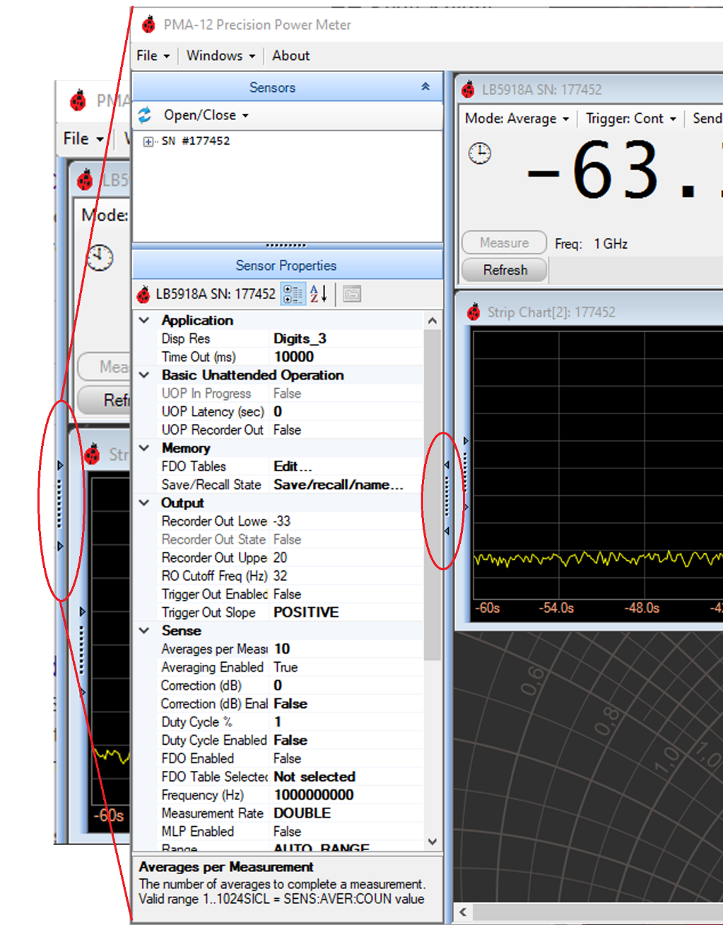
Settings not on the dropdown menus — time-gated measurements, Frequency Dependent Offsets, Recorder Output, and more — live in the Details Pane, opened with the small arrows on the window edge. Some settings appear in both a dropdown and the Details Pane; consult the Programming Guide for anything not covered in this manual.
Trace Mode Controls
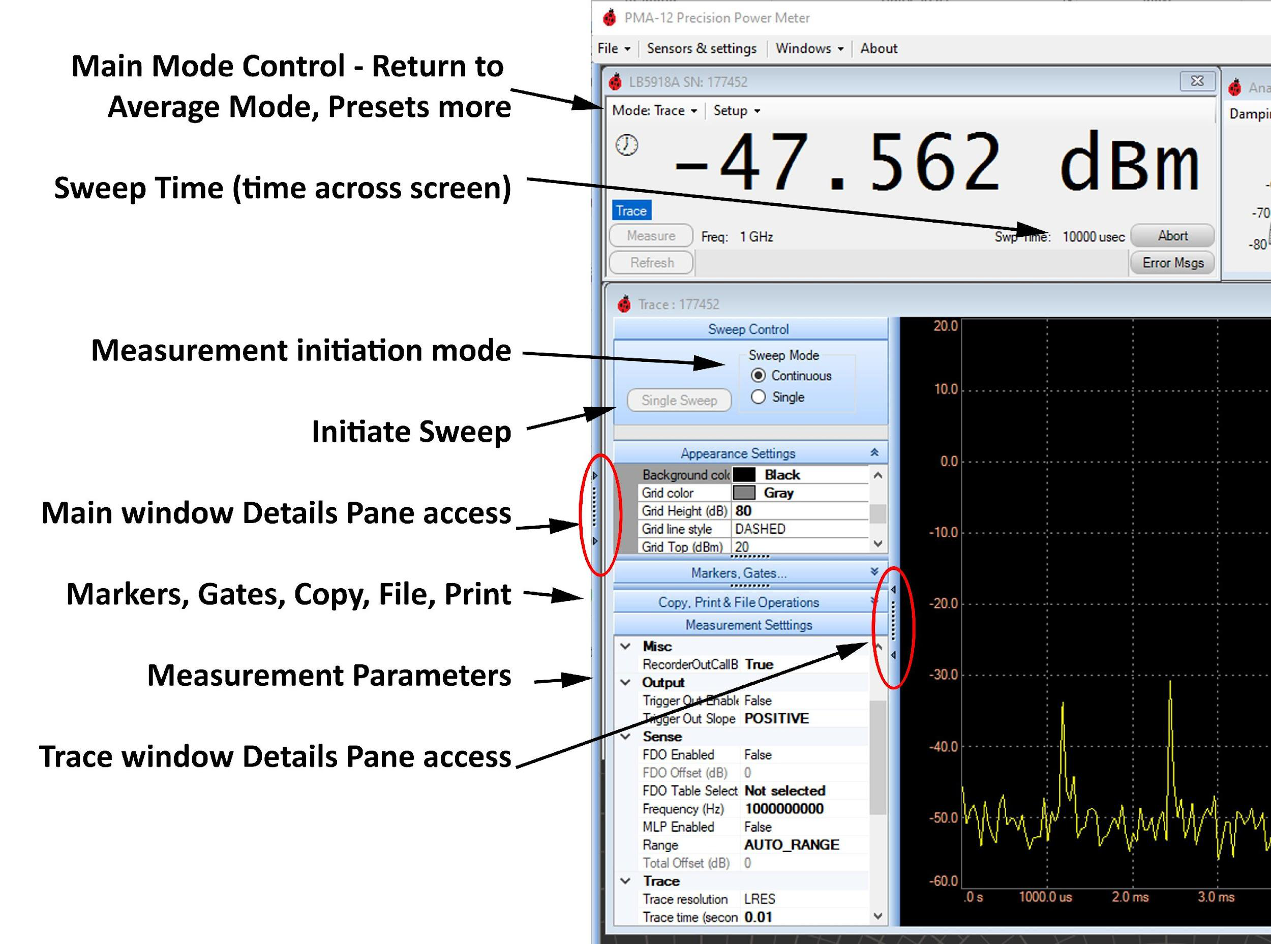
Activating Trace mode places the sensor in Normal Detector mode (see Trace Measurements in Section 2). After PowerEye configures the sensor, the Trace Display appears; return to Average Mode from the Sensor Window's Mode dropdown. Trace time is controlled by Swp Time in the Sensor Window or Trace Time in the Trace Controls Pane — the same parameter either way.
Sweep Control (Trace Initiation)
Continuous initiates a new measurement as soon as the previous one completes (after the trace is delivered); Single waits for manual initiation via the Single Sweep button. Initiation is not triggering — triggering can only occur after a measurement has been initiated.
Trace Appearance Settings
Below Sweep Control in the Trace Detail Pane, these settings change the display's appearance and numeric scales for better detail on a particular level or time range.
Markers, Gates…
Enable a marker, gate, or graphical trigger level from its checkbox in the Markers, Gates… section; each appears on screen and can be adjusted with the mouse. In the checkbox table, Value shows the feature's set point, and for some features (such as Average Gate Power) also a returned measurement. Click a feature's icon to adjust its shape and color.
Trace Copy, Print & File Operations
Copy to Clipboard copies the trace as a list of time and power-level points, pasteable into Excel or other Windows software. Print Image prints the chart in color (adjustable). Save Image to File generates a GIF of the chart. Save Data generates a txt file identical to the clipboard data.
Trace Controls Pane (Measurement Settings)
- Application — Time Out (ms). The default 10 second timeout is adequate for most applications, but some triggered applications may need it changed.
- Memory — FDO & Offsets. Offsets, including MLP and FDO tables, are covered in Section 2; Duty Cycle correction is not available in Trace Mode because the waveform's full period may be unknown.
- Output (Trigger Out). Applied through the sensor's TO SMB connector. If Trigger Out Enabled is True, a 500 ns pulse appears at TO when the sensor triggers; Trigger Out Slope sets polarity (POSITIVE: normally 0 V with a positive 500 ns pulse).
- Sense. Covered in Section 2.
- Trace — Resolution. By default Low Resolution (LRES, 230 points); MRES returns 1,000 points; HRES returns a high-resolution trace sized by trace time and the fast sampling range (USB transfer/processing can take relatively long for HRES).
- Trace — Trace Time. Sets the time the trace covers — for example, a 2 ms triggered trace with a delay to capture an anomaly known to occur somewhere in a 1 ms window.
Trigger. Sweep relates to sensor initiation; triggering controls the measurement after initiation.
- Continuous Trigger. If True, the sensor immediately collects and returns a trace after initiation (a non-triggered measurement controlled by Sweep Control). Set to False to wait for an internal or external trigger before reporting trace data after initiation, which allows pre-trigger data. A USB timeout may need adjustment for triggered measurements.
- Hysteresis (dB). Prevents re-triggering; used only with internal triggering (external triggers are digital). It is the level below (or above, if slope is negative) the trigger level at which another trigger is accepted, set in dB regardless of the display unit.
- Trigger Delay — Trg Delay (s). After initiation, the sensor buffers data; after a trigger, it continues until the measurement completes, then returns data starting at the trigger point plus the delay — a negative delay includes pre-trigger data. A default automatic delay may or may not be sufficient for a given application.
- Trigger Impedance. The external trigger input's selectable load: HIGH (default) is 100 kΩ; LOW is 50 Ω.
- Trigger Slope. Positive triggers on a low-to-high external transition, or when an internal signal reaches the trigger level, re-arming when the input goes low or the internal level drops below trigger level minus hysteresis. Negative triggers on a high-to-low transition, or when the signal falls below the trigger level, re-arming when the input goes high or the internal level exceeds trigger level plus hysteresis.
- Trigger Source. Immediate starts the measurement with no synchronization beyond initiation; External and Internal wait for the respective trigger after initiation (Single or Continuous initiation applies to both) — consider the time-out setting for either.
Unit. Sets the displayed measurement unit, Watts or dBm. Although Unit is a sensor function that affects returned data, some settings are always made in one specific unit regardless of the display unit — noted at each such setting; see the programming guide for detail.
System — Sensor Clock. Sensors with Option UOP can use the sensor's internal clock, set to the host computer's time via Set, then System. The sensor must be in Average Mode (not UOP) to set the clock.
§Contact Us
| Berkeley Nucleonics Corporation | 2955 Kerner Blvd., San Rafael, CA 94901 |
| Phone | (415) 453-9955 or 800-234-7858 |
| info@berkeleynucleonics.com | |
| Web | www.berkeleynucleonics.com |
Model 12100 Series & PowerEye Operating and Service Guide · Rev 2.1
Cited in peer-reviewed research
Independent publications citing this instrument, indexed by Bioz. Citation counts and Bioz Stars ratings are shown live and update as new papers are indexed.