1What is particle image velocimetry?
Particle image velocimetry [PIV] is a noninvasive technique for measuring flow velocities. Unlike point measurement tools such as anemometers, laser Doppler velocimeters, and pitot-static tubes, PIV measures velocity over an entire two-dimensional plane at once without disturbing the flow being studied. Since its development in the 1980s, the technique has become a staple of fluid dynamics research in aerodynamics, biofluidics, combustion, microfluidics, and environmental fluids. In both academia and industry, PIV is a standard tool for measuring planar velocity fields in research and development.
2How does particle image velocimetry work?
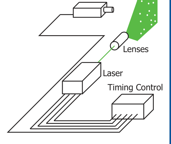
Instead of using an invasive probe, PIV relies on sequential images of visible features within the flow to statistically determine the local velocity. These images must be separated by a short amount of time so that the same visible features in each image are identifiable despite the displacement or deformation imposed by the fluid. To capture these images, a dual-pulsed Nd:YAG or Nd:YLF laser is typically used to illuminate the flow with two brief pulses [Figure 1]. Simultaneously, a high-speed CCD or CMOS camera captures the two illumination pulses in sequential image frames. Since optical access is required for both laser illumination and camera capture, the working fluid is typically transparent and lacks the identifiable features needed for particle image velocimetry.
Due to the lack of inherent tracers, fluid flows are often seeded with particles that follow but do not alter the fluid motion. Spherical particles are often used due to their well understood fluid interactions and visual response to illumination. To enhance their contrast with any fluid or background contaminants, the particles are usually coated to reflect, refract, or fluoresce incident laser light. As the laser fires, the particles in the region of interest are illuminated and produce a tracer field for image capture. For optimal PIV results, the captured images should reveal sharp, point-like particles without any streaking or blurring.
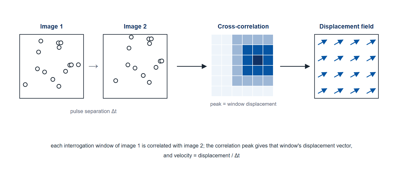
The sequential images of these tracer fields are processed by PIV software to extract the velocity of the fluid flow. To statistically determine the displacement of individual groups of tracer particles, the images are subdivided into smaller pixel groups, known as windows, which are cross-correlated [Figure 2]. This statistical procedure identifies the most probable displacement of the flow tracers from one laser pulse to the next using the pixel pattern of each window on pairs of images. More advanced processing algorithms may include window displacement and deformation to improve the cross-correlation. Once the most probable displacement is known for each window, the velocity field can be calculated using the known separation time between images. Once the velocity field is known, further post-processing may be used to filter the results and produce publication-quality graphics, including velocity vector, vorticity, and streamline plots.
3How does timing affect particle image velocimetry?
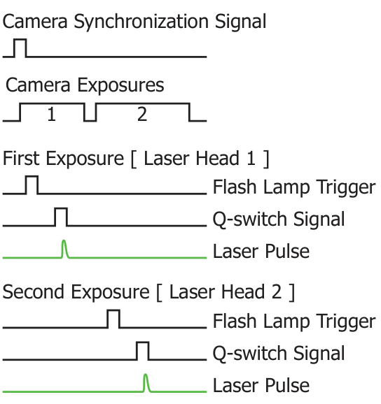
Since repeatable and accurate timing signals are necessary for the collection of reliable particle image velocimetry results, the timing and synchronization requirements can be complex. Dual-pulsed lasers can require up to four signals each to control the pair of synchronized pulses necessary for PIV [Figure 3]. While internal timing can be used to reduce the number of signals required, for complete control of each laser head, a flash lamp trigger to charge the laser and a Q-switch signal to trigger laser pulse emission are needed. By tuning these four separate signals, both the time separation between images and the relative beam intensity are adjustable. A fifth synchronized signal coordinates the camera exposure with the individual laser pulses. If the timing signals activating the laser and camera are not synchronized, the velocity field may be irrecoverable. Even small errors in the timing will lead to errors in the measured velocity field due to its direct reliance on the time separation between pulses. A single device managing every timing pulse keeps the pulse separation, and with it the velocity scale, traceable to one timebase.
4How can BNC meet your timing needs?
Berkeley Nucleonics offers three instruments that manage every PIV timing signal from a single device. The Model 575 and Model 577 Digital Delay/Pulse Generators cover a dual-pulse system from one T0; the Model 725 Multi-Trigger Digital Delay Generator adds programmable logic for experiments whose trigger is a condition rather than an edge.
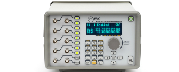
The Model 575 handles the timing of a dual-pulse PIV system from its front panel [Figure 4]. With up to 8 channels, 250 ps delay and width resolution, 50 ps RMS jitter from its internal rate generator, and optional optical inputs and outputs for crossing ground potentials, it controls laser and camera timing along with any other equipment that needs a synchronized trigger, and its onboard interface removes the need to devote computer resources to timing. The Model 577 offers the same 250 ps resolution with 4 or 8 channels, channel-to-channel jitter under 50 ps RMS, repetition rates to 20 MHz, and a 10 to 100 MHz external clock input for locking to a laser oscillator.
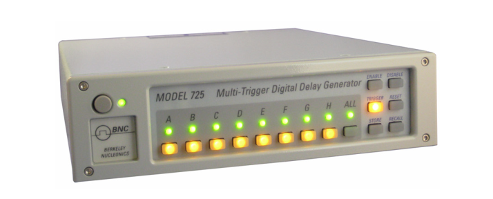
The Model 725 suits PIV experiments where the trigger is a logical condition [Figure 5]. Where the Model 575 references up to 8 channels to one T0, the Model 725 provides eight independently triggered timers with 10 ns resolution and programmable AND, OR, XOR and negated logic between its eight inputs and eight outputs, so a laser can be interlocked to a shutter position or a pressure switch in hardware. It runs stand-alone or under the included timerPRO software, and LabVIEW drivers are available.
One instrument carrying every PIV timing signal removes the cable and clock mismatches that a multi-box setup introduces.